By Albert Gu and Tri Dao.

LLMs are dominated by transformers nowadays. In this blog post we review a different one called Mamba. Mamba has deep ties to the control community, and leveraging wisdom from system control could have potential to improve research on SSM-based large models.

Motivation of Mamba is trying to merge the gap between transformer and a group of more traditional RNN-type models. Essentially, transformer is a type of RNN-type model with expanding hidden state (KV caches), while the traditional RNN-models maintain a fix-size internal state for the whole sequence.

Mamba has competitive performance comparing to transformer at small model level and faster inference speed. But Mamba probably will not replace transformers, and it has the potential to be long-term memory component of the future model architecture.

Basic formulas

Everything starts with the classic continuous-time state-space model

where $x(t)\in\mathbb{R}$ and $y(t)\in\mathbb{R}$ are input and output of the system respectively. This system can be seen as a mapping from $x(t)$ to $y(t)$, via hidden state $h(t)\in\mathbb{R}^N$.

Continuous-time ODEs can only be computed via discretization, which can be formulated as

where

and $\Delta$ is the step size.

Given this discretization (1), the output can be either computed recurrently as in (1), or in convolution as

or more verbosely as

Advantage of doing this is to save the maintain of internal state $h$ which can save some footprint in vram. The authors also discussed that the for efficient training, the convolution form is preferred, but for inference, it mainly use recurrent form.

The classic state-space model is linear time invariant, namely all the matrices are constant which has very limited capability to generalize. Hence the authors proposed the following enhancement of the model architecture.

Structured SSM

Before generalize the weights the SSM (1), the author put one constraint on the matrix $A$ being diagonal for better compute efficiency. Now the matrix $A,B,C$ are essentially N-dim vectors.

Typical token sequences $x$ for LLM is of batch size B, length L and (embedding) channels D. In this case, the SSM is applied to each channel separately, hence the dmension of the total hidden states is DN.

Code realization

The following graph shows the mamba architecture clearly. Here we do a simple inference to understand the flow better. We mainly focus on the class MambaMixer.

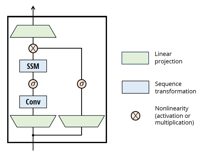
We start with a simple prompt “How are you doing?” with 6 tokens. After embedding layers, the inputs becomes a tensor of shape [1,6, 2560] ([batch_size, seq_len, hidden_size]).

Step 1. Linear projection

# 1. Gated MLP's linear projection
projected_states = self.in_proj(input_states).transpose(1, 2) # [batch, 2 * intermediate_size, seq_len]
hidden_states, gate = projected_states.chunk(2, dim=1)

This part corresponds to the beginning two inverted trapezoids. In paper section 3.4, the author discussed about expansion model dimension D by an expanding factor E. Here the hidden_states and gate will travel through left and right path of the architecture, respectively. We will discuss the gate later when it merge back.

For prefill stage, the hidden_states and gate are of shape [1, 5120, 6] ([batch_size, intermediate_size, seq_len])

For decoding stage, since we generate a new token at a time, the hidden_states is of shape [1, 5120, 1].

Step 2. Convolution

if cache_position.shape[0] == self.conv_kernel_size:  # PREFILL
    conv_state = nn.functional.pad(
        hidden_states,
        (self.conv_kernel_size - hidden_states.shape[-1], 0)
    )

    cache_params.update_conv_state(self.layer_idx, conv_state, cache_position)
    hidden_states = self.act(self.conv1d(hidden_states)[..., :seq_len])  # [batch, intermediate_size, seq_len]
else: # DECODING
    conv_state = cache_params.update_conv_state(self.layer_idx, hidden_states, cache_position)
    hidden_states = torch.sum(conv_state * self.conv1d.weight[:, 0, :], dim=-1)
    if self.use_conv_bias:
        hidden_states += self.conv1d.bias
    hidden_states = self.act(hidden_states).to(dtype).unsqueeze(-1)   # [batch, intermediate_size, 1] : decoding

In paper section 3.5, the authors motivate the convolution by filtering ‘noise’ in long context. Here this convolution part is also selective in the sense that it is input dependent. In other words, the weights of self.conv1d are trainable.

Here in mamba-2.8B model, a convolution kernel of size 4 (conv_kernel_size) is used. For our input sequence which is longer than 4, padding is not needed.

For prefill, the hidden_states after convolution is of shape [1, 5120, 6] ([batch, intermediate_size, seq_len]). The convolution is essentially ‘smooth’ the input sequence.

For decoding, the hidden_states is of shape [1, 5120, 1] before convolution, then the convolution is done with last 4 tokens of the current sequence to generate the output for the current single token. Hence hidden_states after convolution is kept as [1, 5120, 1].

Step 3. SSM recurrent

# 3. State Space Model sequence transformation
# 3.a. Selection:  [batch, seq_len, self.time_step_rank + self.ssm_state_size * 2]
ssm_parameters = self.x_proj(hidden_states.transpose(1, 2))
time_step, B, C = torch.split(
    ssm_parameters, [self.time_step_rank, self.ssm_state_size, self.ssm_state_size], dim=-1
)
discrete_time_step = self.dt_proj(time_step)                                    # [batch, seq_len, intermediate_size]
discrete_time_step = nn.functional.softplus(discrete_time_step).transpose(1, 2) # [batch, intermediate_size, seq_len]

# 3.b. Discretization: B and C to [batch, seq_len, intermediate_size, ssm_state_size] (SRAM)
A = -torch.exp(self.A_log.float())                                              # [intermediate_size, ssm_state_size]
discrete_A = torch.exp(A[None, :, None, :] * discrete_time_step[:, :, :, None]) # [batch, intermediate_size, seq_len, ssm_state_size]
discrete_B = discrete_time_step[:, :, :, None] * B[:, None, :, :].float()       # [batch, intermediate_size, seq_len, ssm_state_size]
deltaB_u = discrete_B * hidden_states[:, :, :, None].float()

# 3.c perform the recurrence y ← SSM(A, B, C)(x)
if self.use_mambapy and self.training and cache_params is None:
    ...
else:
    scan_outputs = []
    for i in range(seq_len):
        ssm_state = discrete_A[:, :, i, :] * ssm_state + deltaB_u[:, :, i, :]      # [batch, intermediade_size, ssm_state]
        scan_output = torch.matmul(ssm_state.to(dtype), C[:, i, :].unsqueeze(-1))  # [batch, intermediade_size, 1]
        scan_outputs.append(scan_output[:, :, 0])
    scan_output = torch.stack(scan_outputs, dim=-1)                                # [batch, seq_len, intermediade_size]
    scan_output = scan_output + (hidden_states * self.D[None, :, None])
    scan_output = (scan_output * self.act(gate))

The is the core part of Mamba, which updates the $h$ according to selective structured SSM (equation (1) in this blog). The first step (3.a) here is to derive the input-dependent (selective) parameters for SSM, namely $\Delta, B, C$. In equation (1), The parameter $\Delta$ controls how much the cuurent input $x_t$ contributes to the SSM state. The authors also use Theorem 1 to motivate that $\Delta$ can be seen as the ‘gating’ mechanism in the traditional RNN domain. In other words, for a special case (scalar integrator), the update of SSM state is weighted average between the previous state and input, and $\Delta$ controls the weight.

Selective vs Learnable. The authors discuss thoroughly about selective mechanism. In short, a variable is selective means it is learnable and input dependent. From the code point of view, the weight matrix A is learnable via

self.A_log = nn.Parameter(torch.log(A))

but weight B, is derived through x_proj which is learnable wrt input (hidden_states)

ssm_parameters = self.x_proj(hidden_states.transpose(1, 2))
time_step, B, C = torch.split(
    ssm_parameters, [self.time_step_rank, self.ssm_state_size, self.ssm_state_size], dim=-1
)

After discretization of the SSM model, the SSM state is updated recurrently. Note that system is maintaining a central SSM state only. The shape of the SSM state of this model is [1, 5120, 16] ([batch_size, intermediate_size, state_size]). The way it updates differentiate by prefill and decoding phases. For prefill, seq_len = 6 (len of our prompt), then the previous (slow) implementation update the SSM state iteratively. For decoding, seq_len = 1 which is only for the newly added token.

Step 4. Output merge

After the recurrent selective SSM, the output are merged with 1. an (internal) residual path from input with (learnable) weights D; 2. gated input

scan_output = scan_output + (hidden_states * self.D[None, :, None])
scan_output = (scan_output * self.act(gate))

Here is the gated path is motivated by transformers MLP layer (for example LlamaMLP). But instead of put gated path after attention block as in transformer, Mamba here take it parallel to SSM. One motivation is to do ‘channel’ filtering (wrt embedding-dim). But could be also simply be that MLP has been working very well in transformers which becomes very risky to skip.

Hardware opt

This paper is written by the author of flash attention, so the hardware efficiency is guaranteed as well. The main idea to keep the heavy lifting of discretization and SSM update in SRAM which is closer to compute unit, while keep the weights $\Delta, A, B, C$ in the HBM and only write back the output y to HBM. This is possible due to the SSM update are independent wrt channels, and can be parallelized by scan algorithm (Blelloch 1990; Martin and Cundy 2018; Smith, Warrington, and Linderman 2023).

Conclusion

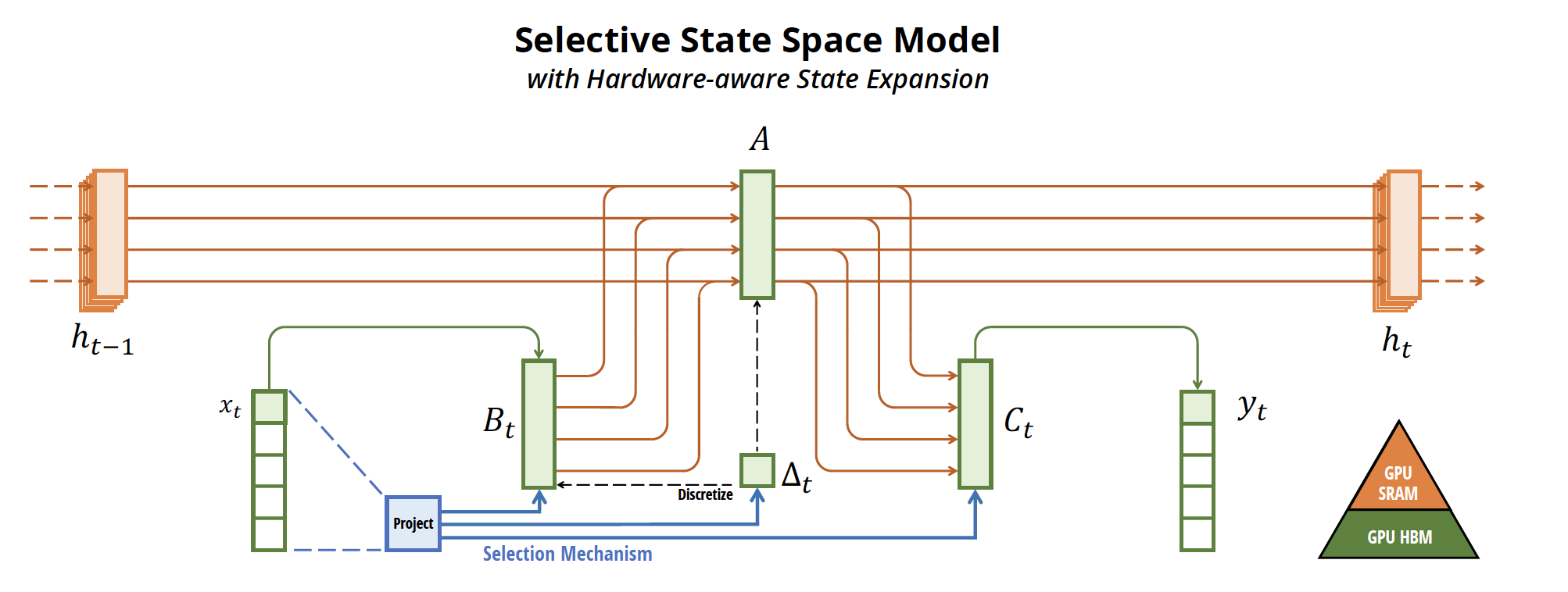
Now this picture makes perfect sense: as the sequence goes on, the latest token is used to update the SSM state recurrently, which will be used further on to generate the next token, and so on.

Since Mamba and transformers are both originated from classic RNN, and they have similarity of their internal tensors, there has been some research showing that some weights of pretrained transformers like Llama can be borrowed to initialize some of the Mamba weights, which in turn saves the training time and gain better performance.

Both advantage and disadvantage of Mamba are pretty clear: it has a fix-size internal state to maintain for infinite-long sequences, which is more efficient transformers with expanding internal states; but because of this information compression, it will loose the details of the long sequences.

Dictionary

Here we collect some key parameters and variable definition from the paper and code. We are using mamba-2.8b for code reference.

This model has 64 hidden layers.

• hidden_size: 2560 (embedding dim, D in paper)
• intermediate_size: 5120 (= 2x hidden_size, ED in paper)
• state_size: 16 (N in paper, config.state_size in code)
• conv_kernel: 4
• vocab_size: 50280
• hidden_state: x in paper