Abstract

The key points of this paper are

• residual connection is ubiquitous. This is a paradigm since ResNet?
• Hyper-Connection extend residual connection
  • can have substantial performance gain
  • but unstable for training
  • hard to scale
  • more memory access overhead
  • this is because HC compromise residual connection’s identity mapping property
• Solution: manifold constrained HC by projecting HC onto a manifold to ensure stability

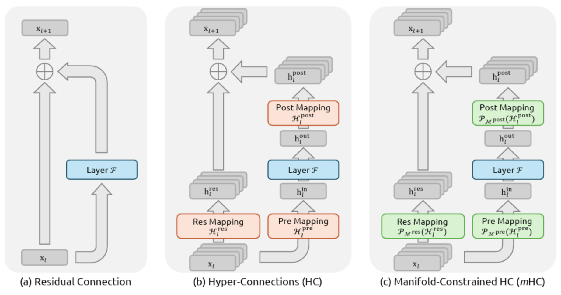
Main Method

The residual connection has been there for deep learning for long time, but has been kept it original form so far. A (probably any) single-layer neural network can be typically formulated as

For simplicity, we can think of $\mathbf{x}_l \in\mathbb{R}^C$. This corresponding to the Transformer with model dimension being $1$.

In fact, for any RNN type of neural network, $\mathbf{x}_l$ is the hidden states of the existing $C$ tokens.

The function $\mathcal{F}(\cdot, \mathcal{W}_{l})$ can be simple matrix multiplication like MLP, or more complicated calculation like attention mechanisms.

Note that when we have multiple layers, the network becomes

namely the input states can come all the way till the end of the network.

Hyper-Connections

This paper is mainly motivated by the paper Hyper-Connections (from Bytedance). The main idea to expand the residual connection, namely one more dimension to the hidden states, and enhance the connection complexity.

Again for simplicity, we take the expansion from 1-D vector to a 2-D matrix, but it can be arbitrary. The formula for HC is

where we have

• $\mathbf{x}_l\in\mathbb{R}^{n\times C}$ is the expanded hidden state and $n$ is the expansion rate
• $\mathcal{H}_{l}^{\text{res}}\in\mathbb{R}^{n\times n}$ is a learnable mapping as feature mixture in the residual connection

In order to keep the remaining part of the neural network unchanged, we need to map $\mathbf{x}_l$ in $\mathcal{F}$ to match the weights $\mathcal{W}_l$. This introduces two more learnable mappings: \(\mathcal{H}_{l}^{\text{pre}}, \mathcal{H}_{l}^{\text{post}}\in\mathbb{R}^{1\times n}\).

Now the multiple layers network with HC becomes

Note that HC has parameterized implementation as

where:

• $\alpha \in \mathbb{R}$ are learnable, initialized to small values
• $\theta_{l}^{\text{pre}}, \theta_{l}^{\text{post}} \in \mathbb{R}^{1 \times C}$ and $\theta_{l}^{\text{res}} \in \mathbb{R}^{n \times C}$
• $\mathbf{b}_{l}^{\text{pre}}, \mathbf{b}_{l}^{\text{post}} \in \mathbb{R}^{1 \times n}$
• $\mathbf{b}_{l}^{\text{res}} \in \mathbb{R}^{n \times n}$ are learnable bias which are initialized to zero (usually).

The author also did an ablation study of HC, and confirms that the expanded residual connection contribute the most to the performance gain.

The contribution of HC is that it not only propose a new residual connection with more stream, but increase the hidden state dimension which can potentially contain more information about a sequence.

The problem of HC is also obvious: it introduces instability with $\prod_{i=1}^{L-l} \mathcal{H}_{L-i}^{\text{res}}$, the elements can be both positive and negative, the eigenvalues are not constrainned etc. Moreover, during the backward propagation, the gradient gain becomes very large (nearly 3000).

mHC

For the system theory and Markov chains, we learned that for autonomous system, governed by a double stochastic matrix, is Lyapunov stable. This is another motivation to the solution proposed by the author. The idea is to map the matrix $\mathcal{H}_{l}^{\text{res}}$ to manifold of stochastic matrices

Note that this manifold is equivalent to the convex hull of all n by n permutation matrix. Also, if the expansion rate $n = 1$, then the manifold is degenerated to $1$, and the residual connection become the classic identity one.

The actual implementation is given as follows.

1. Start with parameterization

where:

• $\vec{\mathbf{x}}_{l}=\text{vec}(\mathbf{x}_{l})\in\mathbb{R}^{1 \times nC}$ is the flattened vector
• $\varphi_{l}^{\text{pre}}, \varphi_{l}^{\text{post}} \in \mathbb{R}^{nC \times n}$ and $\varphi_{l}^{\text{res}} \in \mathbb{R}^{nC \times n^{2}}$ are learnable weights
• $\text{mat}$ is a reshape func from $\mathbb{R}^{1 \times n^{2}}$ to $\mathbb{R}^{n \times n}$

1. Then do the constrained mapping

where $\sigma$ is the sigmoid function and the $\text{Sinkhorn-Knopp}$ operator is working as the following:

1. initialize with

   \[\mathbf{M}^{(0)} = \text{exp}(\tilde{\mathcal{H}}_{l}^{\text{res}})\]

2. iterate

   \[\mathbf{M}^{(t)} = \mathcal{T}_{r}\left( \mathcal{T}_{c}(\mathbf{M}^{(t-1)}) \right)\]

   until converge, where $\mathcal{T}{r}, \mathcal{T}{c}$ are row and column normalization, respectively.

3. denote the final result as

   \[\mathcal{H}_{l}^{\text{res}} = \lim_{t\rightarrow \infty} \mathbf{M}^{(t)}\]

   Practically, take $t_{\max} =20$.

The code implementation of $\text{Sinkhorn-Knopp}$ opt can be as

import torch

def sinkhorn_knopp_torch(X: torch.Tensor, t_max: int = 20) -> torch.Tensor:
    M = torch.exp(X)

    for _ in range(t_max):
        M = M / M.sum(dim=1, keepdim=True)
        M = M / M.sum(dim=0, keepdim=True)

    return M

The benefits of using double stochastic $\mathcal{H}_{l}^{\text{post}}$ are norm preservation which effectively solve the gradient explosion problem; and the residual connection can be seen as a convex combination of information across streams, like a feature fusion mechanism.

why 2 ?

In the mapping of mHC, the factor 2 in post projection is to make the $\mathcal{H}_{l}^{\text{post}}$ close to uniform matrix.

This happens when the elements of $\tilde{\mathcal{H}}_{l}^{\text{post}}$ are close to zero for example at initialization. This is because $\sigma(0) = 0.5$.

Performance

The author did a heaving lifting by implement the kernel fusion to make the training efficient, and experiment with 27B model.

Here are the main results

mHC gives better performance in term of metrics and stability

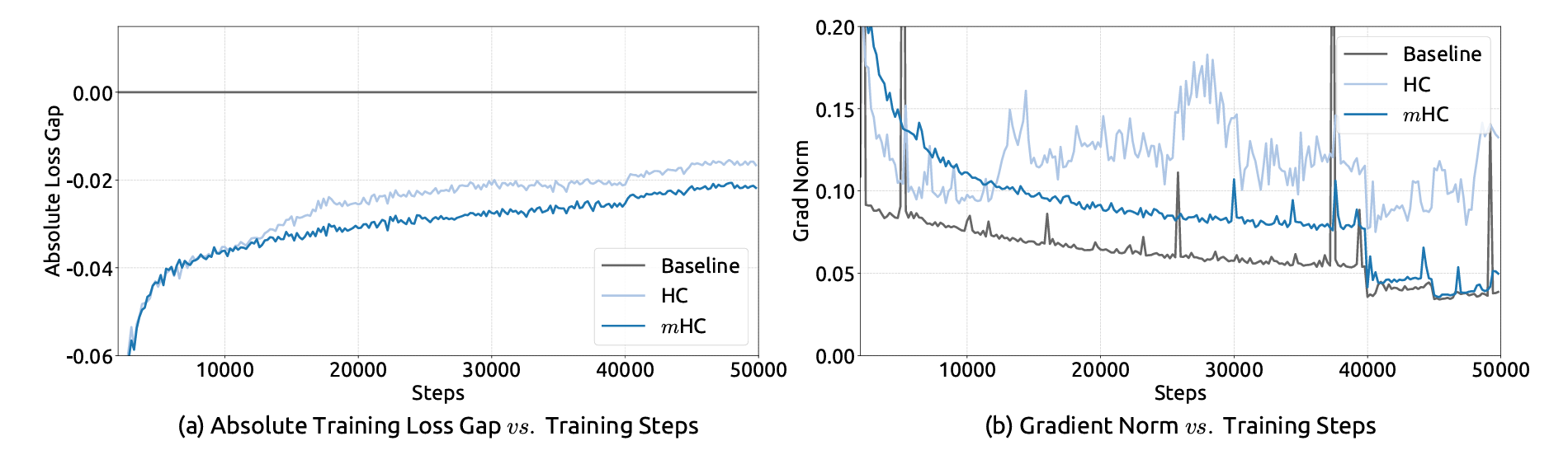
In this figure, we can see that mHC gives the most stable training with the least loss. This is also verified by testing on some benchmarks. mHC outperform the other method in most of the cases.

My takeaway

This is a promising method to expand the overlooked residual connection, which can further more improve of the performance of the Transformer at least. It basically expands the dimension of the hidden state of a neural network. Considering the trend of dimension expansion along RNN (from finite-dimensional hidden states, classic RNN, LSTM, Mamba etc, to infinite-dimensional ones like Transformer), this work opens another perspective to scale.

mHC introduce minor modifications to the other part of the neural network. Except for the Transformer, embedding layers needs to be expanded as well.