Can Repeating Transformer Layers Help?
After reading about looped Transformers and follow-up work like looped transformers in diffusion, training-free methods, here I want to test the idea with relative newer architecture and models: take a pretrained Qwen model with hybrid attention, repeat some of its middle layers, and see whether the extra computation helps.
The same weights are used on every pass. Repeating a block adds computation without adding another copy of its weights. I tried two approaches: train a small model to use the repeated layers, and repeat layers in a larger model without changing its weights (train-free way). The clearest training result came from a task where each pass had a specific job. The training-free results were smaller and depended on the prompt.
First attempt: repeat the layers and fine-tune
Most of the existing work on looped transformer is about full attention model, here I started with Qwen3.5-0.8B, which uses both Gated DeltaNet and full attention. I repeated its middle eight layers. The embeddings, earlier and later layers, and output head stayed frozen.
Qwen3.5-0.8B architecture with frozen front and tail, trained middle layers, and a new trained bridge are given as following figure. The notation is consistent with [9].
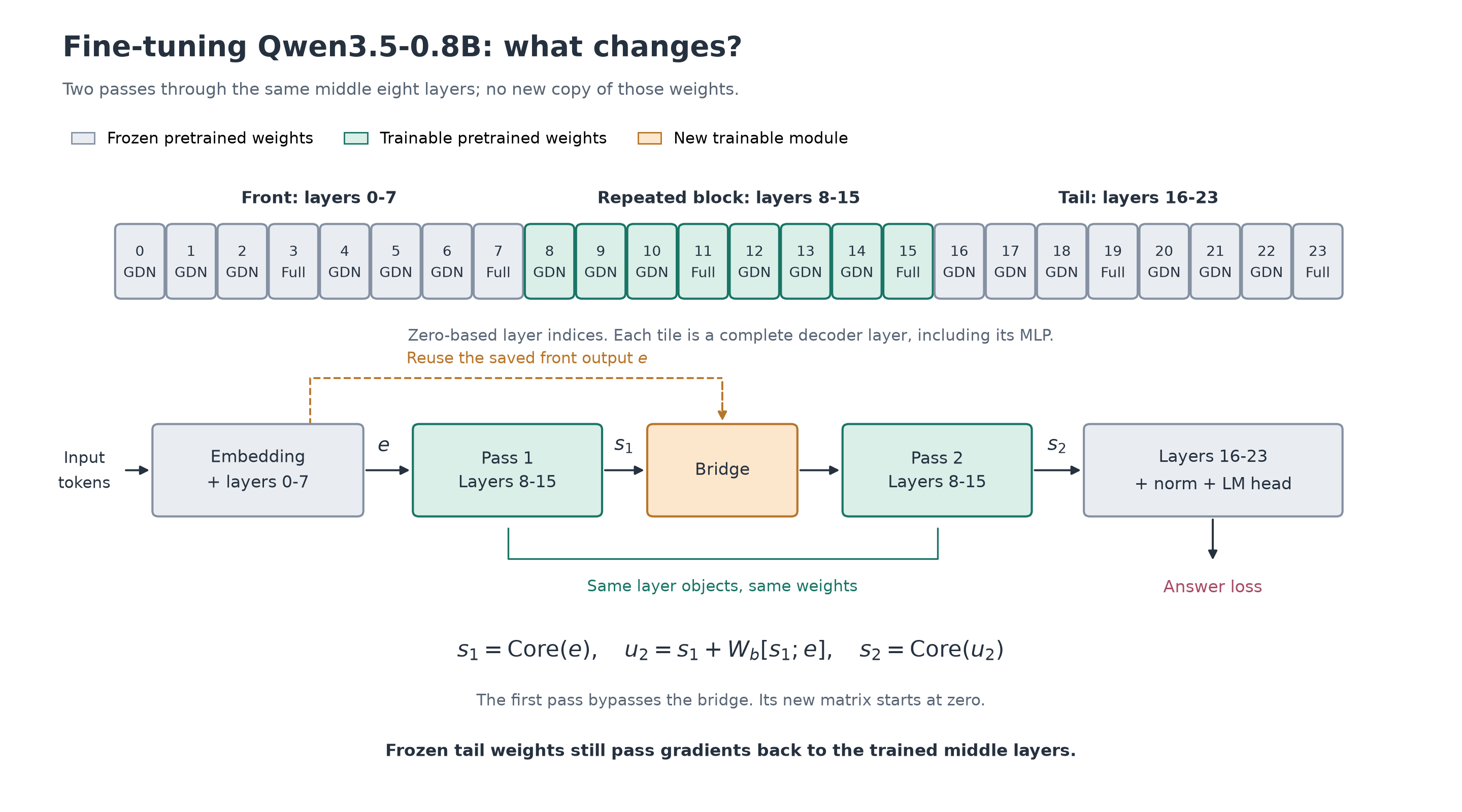
Green: pretrained layers being trained. Orange: the new bridge to merge two input tensors. Grey: frozen weights. Layer indices are zero-based. The two middle blocks share weights.
The first experiment used two passes and 10,000 generated arithmetic examples, trained for one epoch. For comparison, I also fine-tuned a one-pass model on the same examples, in the same order, for the same number of training steps.
One training example was:
Start at 35. Apply these operations in order: add 2, multiply by 2. What is the final number? Answer with only the number. Answer: 74.
Both models learned with the following training loss.
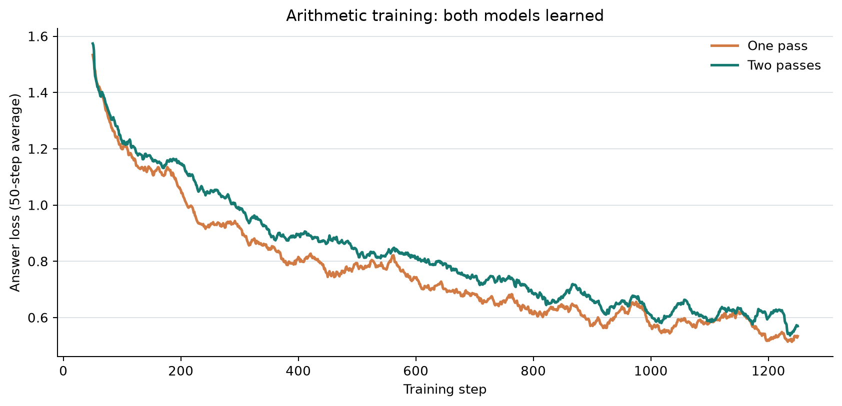
But the training result is not good, two passes did not beat ordinary fine-tuning:
| Evaluation | One-pass fine-tune | Two-pass fine-tune |
|---|---|---|
| 500 questions using the training templates | 42.4% | 38.2% |
| 500 questions with new wording and numbers | 7.4% | 7.2% |
The two-pass model did better when allowed to finish both passes than when stopped after its first pass. That only showed that it used the second pass. It did not show that training with two passes was better than training a separate one-pass model.
Consecutive tasks for the loop
The next experiment is where I could check exactly what each pass/loop should produce. This was inspired by the intermediate-step training in Retrofitting Recurrent Depth into a Pretrained Language Model.
Each question supplies a new rule table over 16 letters, a starting letter, and a number of steps. For example, if the table says A -> L, it maps A to L. Keep looking up the next letter until the requested number of steps is reached.
Calling the table a function (f), the answer after (d) steps is:
\[y_d = f^d(x) = \underbrace{f(f(\cdots f(x)\cdots))}_{d\text{ applications}}.\]During training, pass (i) receives a target of $f^i(x)$. So the first pass learns the first lookup, the second learns the second lookup, and so on. Later in training, I reduced the weight of these intermediate targets and finished with only the final-answer loss. Six passes through shared trained layers, with a frozen readout and a separate target at each pass.
The training process is described in the following plot.
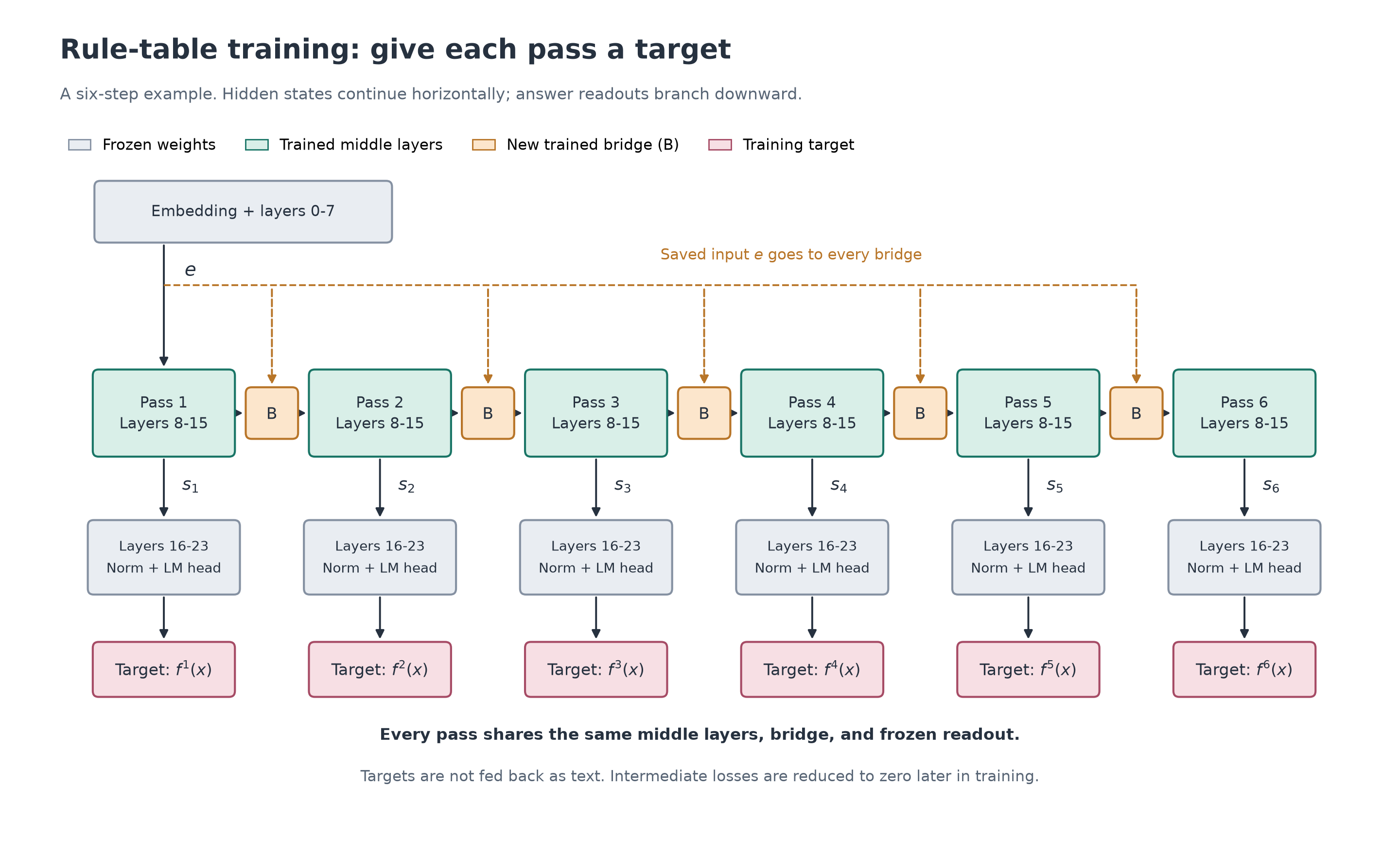
A six-step training example. Shorter (than 6-steps) questions supervise only the passes up to the requested step. The letters are targets, not text fed into the next pass. Here I used a different bridge: learned projections of the previous state and the saved front output, with a learned scalar blend. It is NOT an trainable early-exit gate.
These targets mattered. With the same repeated-layer architecture trained on one to four steps, final-answer accuracy was 213/512 when only the final answer was supervised, compared with 511/512 when intermediate targets were included.
One finding I got is that training on up to four steps did not make the model reliably solve longer chains. I continued training with examples containing up to six steps, then tested on new tables, including seven- and eight-step questions.
Rule-following accuracy by number of required steps
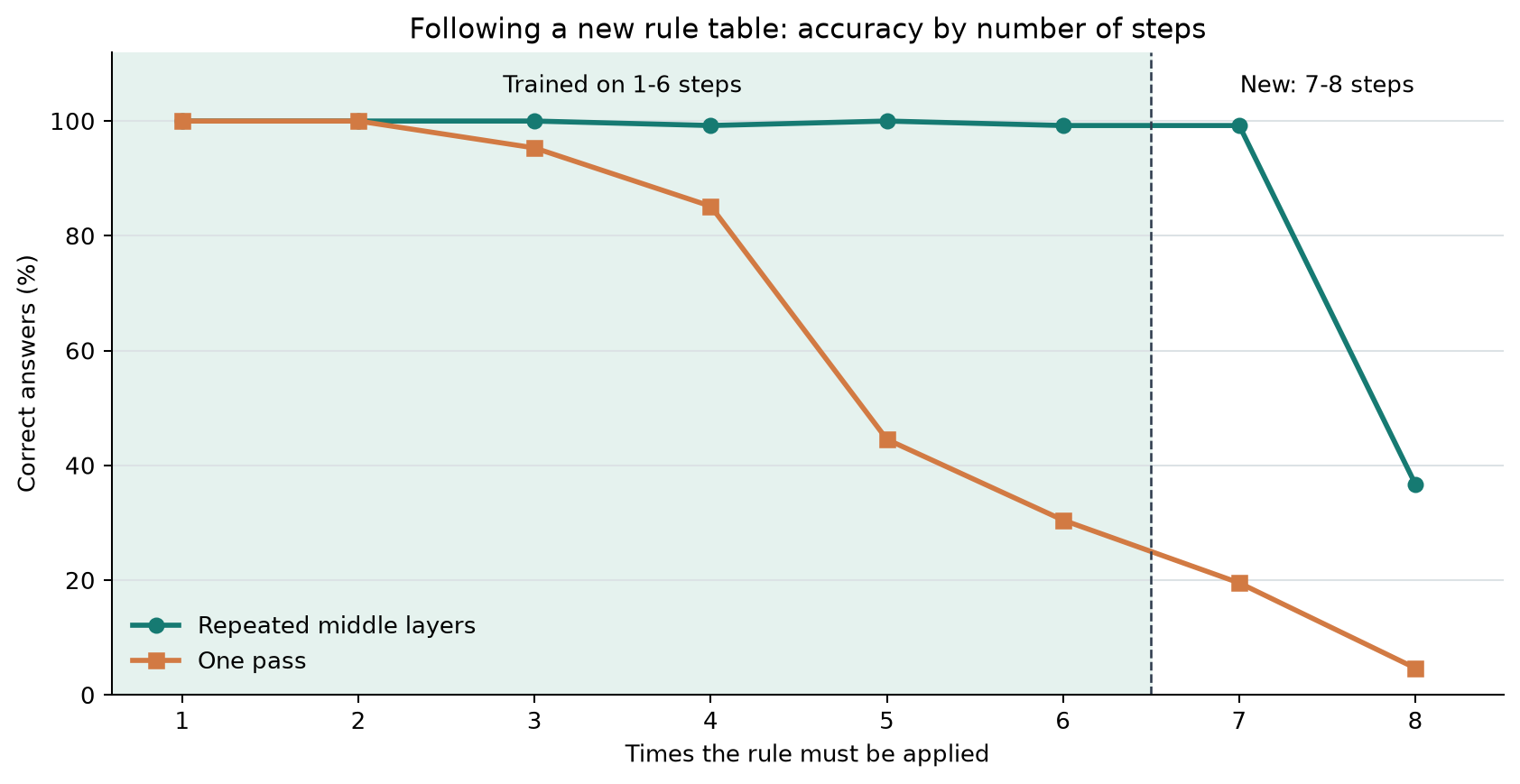
128 questions at each length. The shaded region covers lengths seen during training.
| New test questions | One pass | Repeated middle layers |
|---|---|---|
| 1-6 steps, lengths seen in training | 583/768 (75.9%) | 766/768 (99.7%) |
| 7-8 steps, lengths not seen in training | 31/256 (12.1%) | 174/256 (68.0%) |
One seven-step test question is as follows (provided in the prompt):
B -> M    P -> C    H -> K    I -> E
A -> L    C -> H    G -> L    J -> L
F -> F    L -> E    O -> F    N -> C
D -> B    M -> A    K -> D    E -> P

Start at A. Apply the rule seven times.
The correct path and the model’s answers after each pass were:
| Pass | 1 | 2 | 3 | 4 | 5 | 6 | 7 |
|---|---|---|---|---|---|---|---|
| Correct next letter | L | E | P | C | H | K | D |
| Answer read from the model | L | E | P | C | H | K | D |
The one-pass model answered C; the repeated-layer model reached D.
These letters were read from the hidden states from the each looped layers and decoding layers. They were not generated and fed back as text. The model repeatedly processed its internal representation using the same middle layers.
Does it still work with different wording?
Next, I replaced the compact rule table with sentences, such as Joe's note points to Max. The task was still to start at one person and follow the links a given number of times.
Two models are compared here: the model that had already learned the previous table task, and the original Qwen weights with the same repeated-layer architecture. Both received the same new training data and 1,200 training steps.
Accuracy on new wording across three training runs
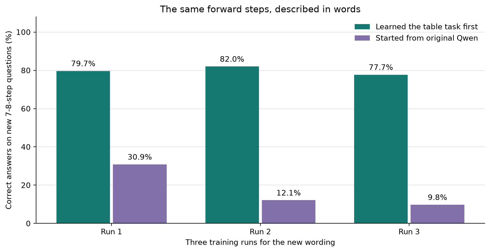
Each run tested 256 new questions requiring seven or eight steps.
The model that first learned the table task scored 79.7%, 82.0%, and 77.7% on seven- and eight-step questions, compared with 30.9%, 12.1%, and 9.8% when starting from the original weights. Learning the repeated operation is helpful in all three runs under the same training budget.
Here it is showing the potential to improve model’s capability on multi-step problems/tasks, including CoT, but with more curated training pipelines.
Repeating layers without training
There has been some work along the training-free path with more computations, e.g., Training-Free Looped Transformers. Here the weights stay frozen. Let $g$ be the selected layer block and $x$ its input hidden states:
\[\begin{aligned} g(x) &= x + F_g(x),\\ F_g(x) &= g(x)-x. \end{aligned}\]The paper views this change as one Euler step to the following ODE:
\[\frac{dx}{dt}=F_g(x).\]Ordinary evaluation takes one unit-sized step. Naively applying $g$ repeatedly takes several full steps, namely stack attention layers repeatedly, which may move the hidden states too far. Instead, take $K$ smaller steps over the same nominal interval:
\[\begin{aligned} x_0 &= x,\\ x_{j+1} &= x_j+\frac{1}{K}\bigl(g(x_j)-x_j\bigr)\\ &=\left(1-\frac{1}{K}\right)x_j+\frac{1}{K}g(x_j),\\ &\qquad j=0,\ldots,K-1. \end{aligned}\]With $K=3$, each pass keeps two-thirds of its input and adds one-third of the block output. With $K=1$, it recovers the original block.
This motivates gentler repeated updates. It does not guarantee better answers: the model was trained as a discrete network, not to reach a known continuous-time solution.
Apply train-free looping to a larger Qwen
I tested above train-free achitecture on Qwen3.8-27B with questions from MMLU-Pro. The setting below repeated four layers, indices 30-33 in zero-based numbering, with three small updates ($K=3$).
Training-free Qwen3.8-27B with all weights frozen and three fixed blended updates through layers 30-33
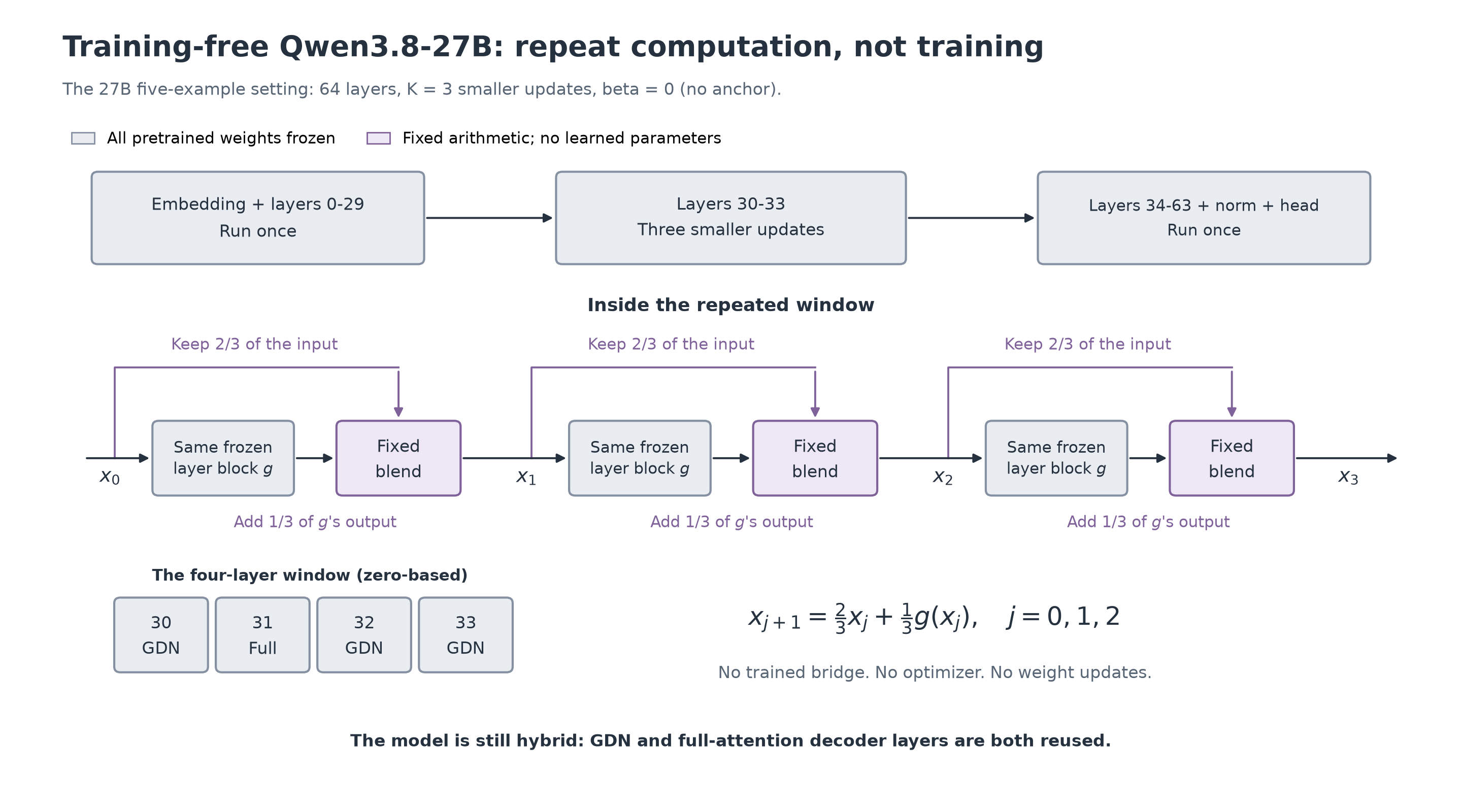
All weights stay frozen. Purple is a fixed weighted sum, not a learned bridge. The repeated window contains three GDN layers and one full-attention layer; both types receive the extra computation.
The model did not generate a chain of thought. I scored the candidate answer letters and selected the highest-scoring one. Chat prompts used the non-thinking setting.
The most interesting results came from adding five answered examples before each question:
| Prompt and subject | Questions | Original | With loops | Difference |
|---|---|---|---|---|
| Engineering, plain prompt | 450 | 58.44% | 57.11% | -1.33 points |
| Engineering, chat with no examples | 450 | 55.11% | 55.11% | 0.00 points |
| Engineering, chat with five examples | 450 | 57.78% | 60.00% | +2.22 points |
| Other subjects, plain prompt | 1,000 | 66.60% | 66.40% | -0.20 points |
| Other subjects, chat with five examples | 1,000 | 66.00% | 67.30% | +1.30 points |
Five examples, or “5-shot”, means five questions from the same subject, each followed by its correct answer letter. This is typical in-context learning setup. The test questions themselves stay the same. Only the context changes; no weights are updated.
For engineering, loops corrected 19 answers and broke 9, giving 10 more correct answers overall. On the other subjects, they corrected 28 and broke 15.
A fresh test with the layers, number of passes, and prompt fixed in advance is still needed. I also tried a small test with actual generated reasoning; it did not improve accuracy. These experiments do not establish that loops can save reasoning tokens at the same answer quality.
Use the earlier passes when decoding
A recent paper from Apple, Decoding Looped Transformers Better for (Almost) Free, suggests why we discard the earlier predictions. Its method, LoopCD, uses an earlier pass to guide the final one without updating the model weights.
There are two methods discussed in this paper.
-
For the same input prefix and next token, let $z_1$ be the first pass’s vocabulary scores and $z_R$ the final pass’s scores. LoopCD-Logits adjusts them as:
\[\begin{aligned} z_{\mathrm{guided}} &= z_R+\omega(z_R-z_1),\\ p_{\mathrm{guided}} &= \operatorname{softmax}(z_{\mathrm{guided}}). \end{aligned}\]The parameter $\omega$ is called strength. The idea is to amplify the change made by the extra passes. With $\omega=0$, this uses the final pass’s logits without guidance; the loops still run. This contrasts predictions for the same token, rather than averaging different generated answers.
-
LoopCD-Hidden instead combines the hidden states before the remaining layers and output head:
\[h_{\mathrm{guided}}=h_R+\omega(h_R-h_1).\]
The logits version needs an extra readout of the earlier state. The hidden-state version keeps one readout, adding only a small vector operation.
In the adaptive logits method, cap is the maximum strength, $\omega_{\max}$. So cap 1 means $\omega_{\max}=1$, not a fixed $\omega=1$; the actual strength changes with the model’s uncertainty.
I tested both versions on the frozen hybrid Qwen3.8-27B. The first test used three small updates and five answer-only examples, without generating reasoning:
| Method | New MMLU-Pro (520 questions) | Earlier engineering set (450 questions) |
|---|---|---|
| Original Qwen | 65.77% | 57.78% |
| Loops without guidance | 66.15% | 60.00% |
| LoopCD logits, strength 0.5 | 66.54% | 59.33% |
| LoopCD adaptive logits, cap 1 | 66.73% | 58.22% |
| LoopCD hidden, strength 0.5 | 66.92% | 59.78% |
The new MMLU-Pro questions showed small positive changes, but the paired uncertainty intervals included no improvement. The earlier engineering set had already been examined and did not show the same pattern.
The paper’s Looped-Qwen3 uses frozen full-attention Qwen3-4B. Here the main experiments use Qwen3.8-27B with Gated DeltaNet plus full attention (27B configuration). The looping idea is shared, but these are different backbones and not an exact reproduction.
Another recent reference, Looped Diffusion Transformer, takes the idea into image generation: shared blocks repeat inside each denoising step, with training supervision on intermediate loops and attention updates designed to stay stable.
The conclusion
The strongest result was on a task with an explicit repeated operation: follow a newly supplied rule, one step at a time. Intermediate targets helped the model learn what each pass should do, and it could then handle some longer chains and new wording.
The training-free approach avoids changing the weights. It gave a smaller positive signal with five examples in the prompt, alongside several flat or negative results. Still need more testing to confirm this as improvement.
References
- Training-Free Looped Transformers. The residual-update motivation and training-free algorithm; see Section 2.3.
- Retrofitting Recurrent Depth into a Pretrained Language Model: Installation, Extrapolation, Transfer, and Retention at Two Parameter Budgets. Inspiration for training with intermediate targets and checking longer chains and retained abilities.
- Qwen3.5-0.8B model card.
- Qwen3.8-27B model card.
- MMLU-Pro. The public multiple-choice benchmark used in the training-free tests.
- Think you have Solved Question Answering? Try ARC, the AI2 Reasoning Challenge. The benchmark used to check performance after fine-tuning.
- Looped Diffusion Transformer. Repeated Transformer blocks within diffusion denoising steps, with intermediate supervision and attention regulation.
- Decoding Looped Transformers Better for (Almost) Free. LoopCD uses earlier recurrent predictions to guide decoding in logit or hidden-state space.
- Scaling up Test-Time Compute with Latent Reasoning: A Recurrent Depth Approach
Enjoy Reading This Article?
Here are some more articles you might like to read next: