From Traditional Attention to hybrid ones

1. Traditional Softmax Attention

At token $t$, standard causal self-attention calculates the similarity between the current query $q_t$ and every previous key $k_i$:

\[a_{ti} = \frac{ \exp(q_t^\top k_i) }{ \sum_{j=1}^{t}\exp(q_t^\top k_j) }\]

The output is the weighted sum of all previous values:

\[o_t = \sum_{i=1}^{t}a_{ti}v_i = \frac{ \sum_{i=1}^{t}\exp(q_t^\top k_i)v_i }{ \sum_{i=1}^{t}\exp(q_t^\top k_i) }\]

In matrix form $O=\operatorname{softmax}(QK^\top)V$. A future query will do this match towards any previous key. Therefore, the model normally keeps every previous key and value:

\[\begin{aligned} K_{1:t} &= [k_1,\ldots,k_t],\\ V_{1:t} &= [v_1,\ldots,v_t]. \end{aligned}\]

The KV cache grows with sequence length $O(Ld)$. Linear attention replaces or approximates softmax with a factorable kernel:

\[\exp(q^\top k) \quad\Longrightarrow\quad \phi(q)^\top\phi(k)\]

Here, $\phi$ is a feature map. The attention output can then be written as:

\[o_t = \frac{ \sum_{i=1}^{t} \left( \phi(q_t)^\top\phi(k_i) \right)v_i }{ \sum_{i=1}^{t} \phi(q_t)^\top\phi(k_i) }\]

Using the associativity of matrix multiplication, define:

\[S_t = \sum_{i=1}^{t} v_i\phi(k_i)^\top\]

and the normalization state:

\[z_t=\sum_{i=1}^{t}\phi(k_i)\]

The output becomes:

\[o_t = \frac{ S_t\phi(q_t) }{ z_t^\top\phi(q_t) }\]

Now instead of storing every historical $k_i$ and $v_i$, the model only needs to update two recurrent states:

\[\begin{aligned} S_t &= S_{t-1}+v_t\phi(k_t)^\top,\\ z_t &= z_{t-1}+\phi(k_t). \end{aligned}\]

This can be simplified as linear case:

\[\begin{aligned} S_t &= S_{t-1}+v_tk_t^\top,\\ o_t &= S_tq_t. \end{aligned}\]

where the state has a fixed shape $S_t\in\mathbb{R}^{d_v\times d_k}$ and does not depend on the sequence length. Here the information or memory of the sequence are compressed into the state variable $S_t$.

3. The Limitation of Basic Linear Attention

Basic linear attention only accumulates information:

\[S_t=S_{t-1}+v_tk_t^\top\]

It does not have an explicit mechanism for deleting or overwriting existing information. If similar keys appear multiple times, their values accumulate in the same state. This can cause memory collisions, difficulty removing outdated information, failure to overwrite an existing key-value association, declining retrieval quality as the sequence grows, which are commonly seen in information compression.

4. From Linear Attention to DeltaNet

DeltaNet first uses the current key to retrieve the value already stored in the previous state:

\[v_t^{\text{old}} = S_{t-1}k_t\]

The current token provides a new target value through the value projection:

\[v_t=W_Vx_t\]

The difference between the new value and the retrieved old value is:

\[\Delta v_t = v_t-S_{t-1}k_t\]

Instead of directly adding $v_tk_t^{\top}$, DeltaNet writes only this prediction error:

\[S_t = S_{t-1} + \beta_t \left( v_t-S_{t-1}k_t \right)k_t^\top\]

Expanding the equation gives:

\[S_t = S_{t-1} \left( I-\beta_tk_tk_t^\top \right) + \beta_tv_tk_t^\top\]

Here, $\beta_t\in(0,1)$ controls the ‘writing strength’. DeltaNet provides a key-specific correction: it changes the memory primarily along the direction represented by $k_t$.

5. From DeltaNet to Gated DeltaNet

DeltaNet can precisely update a key-value association, but it has no efficient mechanism for globally forgetting old information. Gated DeltaNet introduces an input dependent decay gate $\alpha_t\in(0,1)$. It first decays the previous memory:

\[\widetilde{S}_{t-1}=\alpha_t S_{t-1}\]

Then it applies the delta update to the decayed state:

\[S_t = \widetilde S_{t-1} + \beta_t \left( v_t-\widetilde S_{t-1}k_t \right)k_t^\top\]

Substituting $\widetilde S_{t-1}=\alpha_tS_{t-1}$ gives:

\[S_t = \alpha_tS_{t-1} + \beta_t \left( v_t-\alpha_tS_{t-1}k_t \right)k_t^\top\]

An equivalent form is:

\[S_t = S_{t-1} \left( \alpha_t \left( I-\beta_tk_tk_t^\top \right) \right) + \beta_tv_tk_t^\top\]

Here the two gates have different responsibilities. $\alpha_t$ is about how much of the previous memory should be retained; $\beta_t$ is about how strongly the current key-value association should be updated The query reads information from the updated state $o_t=S_tq_t$. Here both $\alpha_t$ and $\beta_t$ are input dependent. A key difference between gated DeltaNet and classic attention is that a pure Gated DeltaNet layer does not need a token-level KV cache that grows with the context length. During inference, it just need to keep the recurrent state:

\[S_t\in\mathbb{R}^{d_v\times d_k}\]

It also keeps the most recent (K-1) activations required by the short causal convolution. Its persistent inference state is approximately $O(d_vd_k+Kd)$ where K is the fixed convolution kernel size. In comparison, full attention cache is of scale $O(Ld)$. However, the fixed state is a lossy compression of the sequence.

7. Why Use a Hybrid Architecture?

Pure Gated DeltaNet is efficient, but the capacity of its fixed-size state is limited. Full attention provides stronger token-level retrieval, but its KV cache grows with context length. To remedy this, recent models therefore commonly use a hybrid architecture by combining gated DeltaNet and full attention. One well-known architecture is Kimi K3, which employs an modified Gated DeltaNet, i.e., Kimi Delta Attention. Kimi Delta Attention (KDA) extends Gated DeltaNet by replacing the single scalar decay gate with a vector-valued, channel-wise gate:

\[\alpha_t \in (0,1)^{d_k}, \qquad D_t = \operatorname{Diag}(\alpha_t)\]

Using the state convention of this page, where $S_t \in \mathbb{R}^{d_v \times d_k}$, the update can be written as:

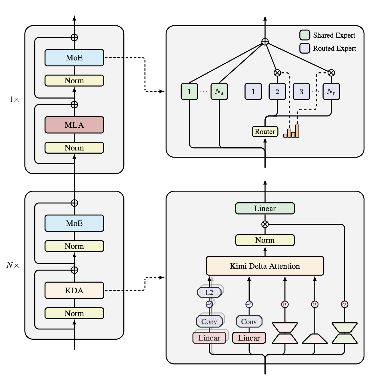
\[S_t = S_{t-1}D_t\left(I-\beta_t k_tk_t^\top\right) + \beta_t v_tk_t^\top\]

(The Kimi paper uses the transposed state convention, so its matrix order appears reversed.) In Gated DeltaNet, one scalar controls how quickly the entire state of a head decays $\alpha_t S_{t-1}$. In KDA, every state channel has its own retention rate $S_{t-1}D_t$. This allows some channels to preserve information for longer while others are updated or forgotten quickly. It makes the fixed-size recurrent memory more expressive. Kimi Linear is a hybrid model, which interleaves three KDA blocks with one Multi-Head Latent Attention (MLA) block $\text{KDA} \rightarrow \text{KDA} \rightarrow \text{KDA} \rightarrow \text{MLA}$. Here only the MLA layers require a sequence-growing KV cache. With this 3:1 ratio, Kimi Linear reduces KV-cache usage by up to ~75% compared with an all-MLA model. Each block still includes a channel-mixing MoE/FFN sublayer after its token-mixing sublayer. KDA or MLA replaces the attention operation, not the entire Transformer block. The architecture can be shown as follows.

Experiments

I compared Qwen3.5-35B-A3B-FP8 with Qwen3-30B-A3B-FP8 on one A100-SXM4-80GB using vLLM 0.18.0. Qwen3.5 contains 30 GDN layers and 10 full-attention layers, while the Qwen3 baseline contains 48 full-attention layers. Since they are separately trained models, here we are looking for a practical systems comparison, not an ablation.

Context	Qwen3.5	Qwen3	Cache saving	TTFT speedup
1K	81.4 MiB	96 MiB	15.2%	0.75x
4K	141.4 MiB	384 MiB	63.2%	1.04x
8K	221.4 MiB	768 MiB	71.2%	1.17x
16K	381.4 MiB	1,536 MiB	75.2%	1.37x
32K	701.4 MiB	3,072 MiB	77.2%	1.69x

The following figures show attention-cache scaling and system performance as context length increases.

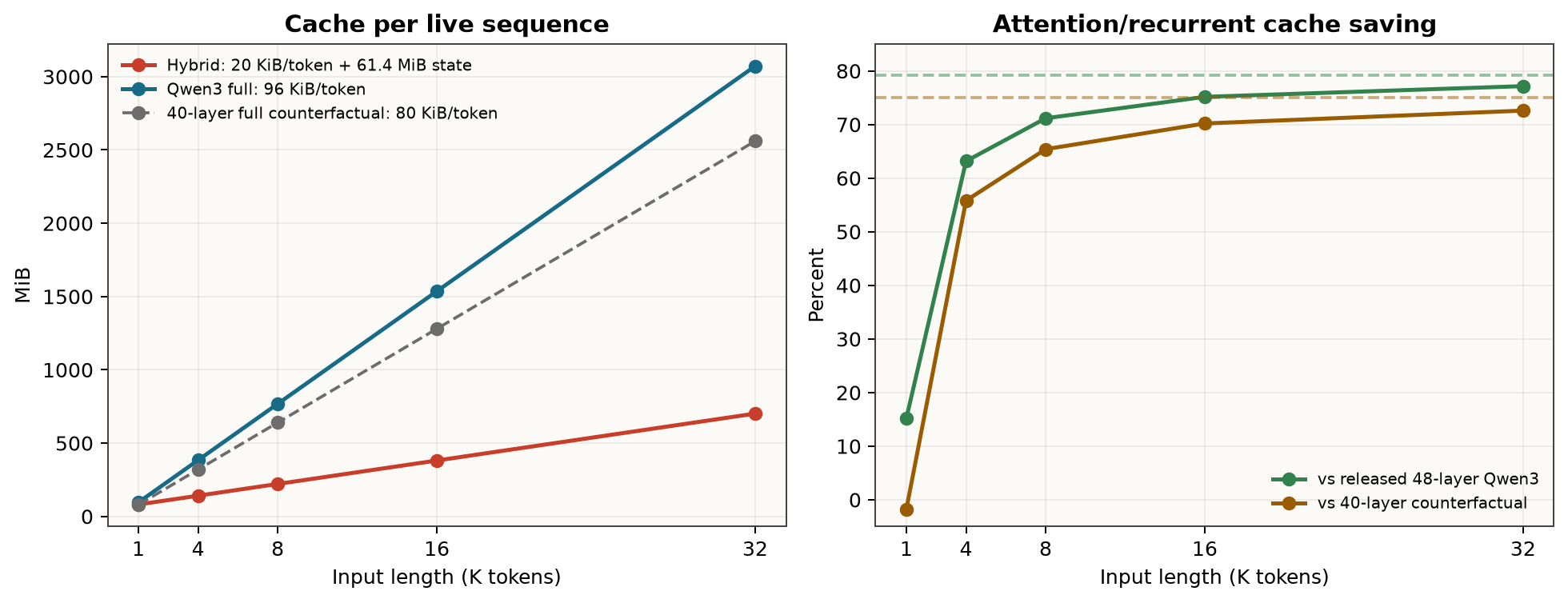
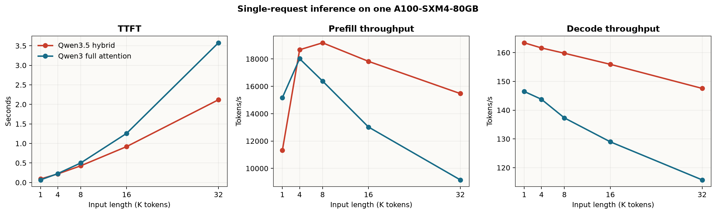
The fixed GDN state is noticeable at short context: at 1K, Qwen3.5 saves little cache and has worse TTFT. Around 4K the latency crosses over; at 32K, its attention cache is 77.2% smaller than the Qwen3 baseline and TTFT is 1.69x faster.

vLLM Storage: GDN State vs. Full-Attention KV Cache

For a hybrid model such as Qwen3.5, vLLM maintains two different kinds of inference state:

• Full-attention layers cache the key and value of every previous token. This state grows with context length.
• GDN layers do not retain token-level K/V pairs. Each live sequence keeps a fixed recurrent matrix state, plus the most recent activations required by the short causal convolution.

\[\begin{aligned} M_{\mathrm{full}}(L) &= O(Ld),\\ M_{\mathrm{GDN}} &= O(d_vd_k+Kd). \end{aligned}\]

In vLLM’s Mamba-style cache interface, ssm_state stores the GDN recurrent matrix and conv_state stores the short Conv1D history. The name ssm_state is an implementation convention; it does not mean that a separate Mamba or classical SSM runs beside GDN. Therefore, only the full-attention part of a hybrid model has cache memory that grows with sequence length. The GDN state is fixed per live sequence and updated in place.

Looped Transformers: Two Recurrent-Depth Architectures

In this section, we review two looped transformers architectures. Both models increase effective depth by repeatedly applying Transformer layers with shared weights. The main idea is similar, but the recurrent units are different.

1. Huginn

The model is divided into a non-recurrent Prelude, a small recurrent Core, and a non-recurrent Coda:

\[\begin{aligned} e &= P(x),\\ s_0 &\sim \mathcal{N}(0,\sigma^2 I),\\ s_i &= R_\theta(e,s_{i-1}), \qquad i=1,\ldots,r,\\ y &= C(s_r). \end{aligned}\]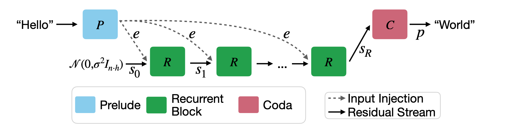

Figure. Huginn’s Prelude-Core-Coda architecture. The Prelude computes the input representation $e$ once; every shared recurrent block receives both the evolving state $s_{i-1}$ and the same input representation $e$; the Coda decodes the final state $s_r$.

The original input representation is injected into every recurrence:

\[s_i=R_\theta\left(A[s_{i-1};e]\right)\]

For the large model, the layer allocation is:

\[(l_P,l_R,l_C)=(2,4,2)\]

Therefore, with recurrence depth $r$, the effective depth is:

\[D_{\mathrm{eff}}=2+4r+2\]

Training samples $r$ from a heavy-tailed distribution with mean $\bar r=32$, giving an average effective depth of approximately 132 layers.

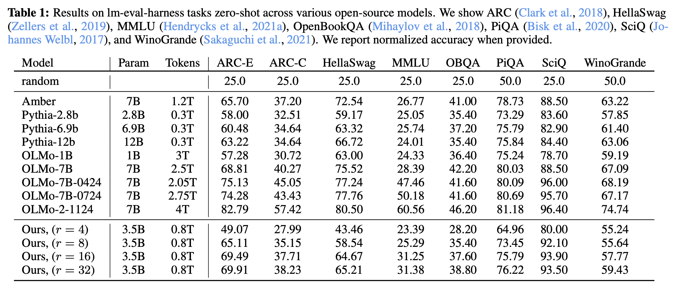
The main experimental result of Huggin is test-time recurrence scaling: the same model becomes stronger when it is allowed to perform more internal latent computation. This is not a state-of-the-art result, but it shows that latent depth can serve as another test-time compute axis alongside Chain-of-Thought in words/tokens.

2. Ouro

Ouro from Bytedance treats the entire Transformer stack as the recurrent unit:

\[\begin{aligned} h_0 &= \operatorname{Emb}(x),\\ h_i &= \mathcal{M}_\theta(h_{i-1}), \qquad i=1,\ldots,T,\\ p_i &= \operatorname{softmax}\!\left(\operatorname{LMHead}(h_i)\right). \end{aligned}\]

Here, $\mathcal{M}_\theta$ is a complete 24-layer Transformer stack. The same 24 layers are reused for every loop. With $T=4$ loops:

\[D_{\mathrm{eff}}=24\times4=96\]

Unlike Huginn, Ouro does not explicitly re-inject the original embedding at every loop. Each loop directly refines the hidden state produced by the previous loop.

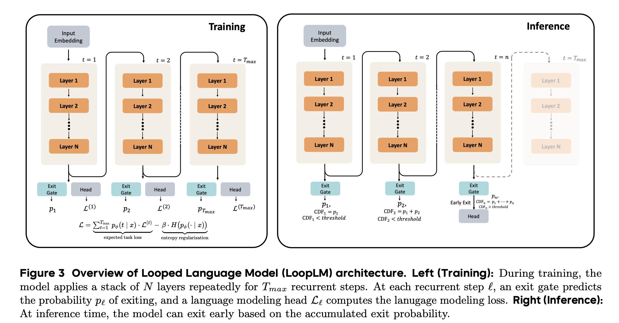
In above figure, every recurrent step produces both an LM prediction and an exit probability during training. During inference, the same forward process is repeated only until the accumulated exit probability crosses a deployment threshold.

Adaptive Exit Gate

At recurrent step $t$, a small linear head reads the current hidden state and predicts the conditional probability of exiting now:

\[\lambda_t(x)=\sigma\left(\operatorname{Linear}_{\phi}(h^{(t)})\right)\]

The probability of surviving the first $t$ loops without exiting is:

\[S_t(x)=\prod_{j=1}^{t}\left(1-\lambda_j(x)\right)\]

Therefore, the probability of exiting for the first time at step $t$ is:

\[p_{\phi}(t\mid x)=\lambda_t(x)S_{t-1}(x)\]

The remaining probability mass is assigned to the final loop. At inference, Ouro exits at the first step whose cumulative exit probability crosses a threshold $q$:

\[t_{\mathrm{exit}} = \min\left\{ t:\; 1-\prod_{j=1}^{t}\left(1-\lambda_j(x)\right)\ge q \right\}\]

A smaller $q$ favors lower latency; a larger $q$ permits more latent computation.

Main Engineering Challenge

Adaptive depth creates a variable execution path. Different requests—and potentially different tokens—may stop after different numbers of loops. For example, easy request may exit after loop 1, while more difficult ones may need full loop 4. GPU inference systems obtain high utilization by batching requests through the same kernels, CUDA graphs, and predictable KV-cache operations. Dynamic exits can cause the batch to diverge. Padding every request to the deepest loop removes most of the speed benefit, while repeatedly splitting or compacting batches introduces scheduling overhead and fragmentation. Current inference frameworks are much better suited to a fixed loop count than true token-level adaptive recurrence.

Fixed-Exit Smoke Test

Here I ran Ouro-1.4B on a small arithmetic problem:

A teacher buys 6 boxes of notebooks with 8 notebooks in each box. She gives 13 notebooks to students. How many notebooks remain?

The correct answer is:

\[6\times 8-13=35\]

The same checkpoint was decoded from each fixed recurrent state:

exit_at_step	Recurrences represented by selected state	Effective depth	Generated answer
0	1	24 layers	10
1	2	48 layers	31
2	3	72 layers	35
3	4	96 layers	35

The first two recurrent states produce incorrect answers. The third recurrence changes the answer to the correct value, and the fourth retains it. This is a concrete example of latent recurrent depth improving a prediction without adding visible Chain-of-Thought tokens.

References

1. Gated Delta Networks: Improving Mamba2 with Delta Rule - gated delta updates, fixed recurrent state, and chunkwise parallelism.
2. Kimi Linear: An Expressive, Efficient Attention Architecture - Kimi Delta Attention and the KDA/MLA hybrid architecture.
3. Qwen3 Technical Report - the Qwen3 model family.
4. Qwen3-Next: Towards Ultimate Training & Inference Efficiency - the hybrid GDN/full-attention architecture on which Qwen3.5 builds.
5. Qwen3.5: Towards Native Multimodal Agents - the official Qwen3.5 release and architecture overview.
6. Scaling up Test-Time Compute with Latent Reasoning - Huginn’s Prelude-Core-Coda recurrent-depth architecture.
7. Scaling Latent Reasoning via Looped Language Models - Ouro’s looped Transformer and adaptive exit mechanism.