KV Cache Management: Quantization and Compression

Motivation

In the (causal) self-attention part of the transformer, the attention output is calculated as

\[\mathrm{Attention}(Q, K, V) = \mathrm{softmax}\left(\frac{Q K^{\top}}{\sqrt{d_k}}\right) V\]

where Q K V are computed by linear mapping from hidden state by corresponding weight matrices. During prefilling, all these Q K V are computed all in same layer at the same forward pass. However, during decoding, at the end of the existing sequence, the last token needs to calculate its attention to all previous tokens. Hence, instead of re-compute the previous K V, these tensors are typically cached.

The formula for KV cache memory usage is

\[2 \cdot \text{precision} \cdot n_{\text{layers}} \cdot d_{\text{model}} \cdot \text{seqlen} \cdot \text{batch}\]

where 2 is for two matrices (K and V), precision is bytes per parameter (4 for fp32), the rests are model parameters. For example, for a 48-layer model, $d_{\text{model}}$=7168, fp16 for inference, and sequence with 1024 tokens, a batch size 128, the total KV cache takes 180 GB vram, while model itself only takes 60GB.

KV cache compression

Not all the tokens are important. Early work e.g. [1] find empirically that, start from prefill and through out decoding, LLM has a persistence manner to pay attention to a subset of token repetitively. Then the authors in [1] proposed ‘Scissorhands’ algorithm for KV cache compression, which is one of the pioneer work in this field.

Top-k attention

Another early work [2] which is not about KV compression, showcased the attention matrix (prefilling for inference, or training/fine-tuning) can be compressed by only kept the most important attention score. The compression is done by row-wise, i.e., for each query vector, it only keeps its k largest similarity scores. In formula

\[\operatorname{top-}k\text{-}\operatorname{Attention}(Q,K,V) = \operatorname{activation}\bigl(\operatorname{top-}k(QK^{\top})\bigr)\,V,\]

which makes the final attention matrix be sparse. The paper provided forward and backward algorithm to incorporate this change into training, and also did plug-in test for inference only. While it saves the storage, the computation of top-k can be a bottleneck for many accelerators.

SnapKV

This work [3] is an important milestone for KV cache compression, especially for long prefill sequence, e.g., long agentic tool results analysis, multi-layer skills, etc. This paper answers (positively) two crucial questions:

1. Is there a consistent attention allocation pattern for input sequence tokens?
2. Is it feasible to identify this pattern prior to the generation stage?

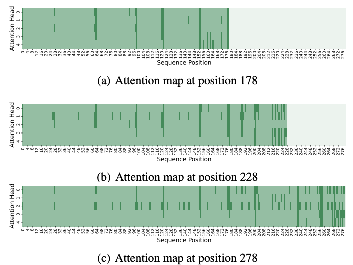
The attention allocation of most input sequence tokens stay consistent during generation. Thus, LLMs knows what you are looking for, and what to say, before generation.

The author showcased that each head consistently focuses on specific prompt attention features (could be a single token, could be a cluster, etc) during generation. Moreover, this robust pattern can be obtained from an ‘observation’ window located at the end of prompt.

Algorithm in detail

1. Denote the input sequence length as $L_{\mathrm{prompt}}$
2. The prompt is partitioned into segments every say 128 tokens. Observation Window is the last segment with length $L_{\mathrm{obs}}$
3. The sequence before the observation window is denoted as prefix with length $L_{\mathrm{prefix}}$, i.e., $L_{\mathrm{prompt}} = L_{\mathrm{prefix}} + L_{\mathrm{obs}}$
4. Voting mechanism:

\[\begin{aligned} \mathbf{C} &= \sum_{i=0}^{L_{\mathrm{obs}}} \mathbf{W}_{\mathrm{obs}}[:, i, :] \\ I &= \operatorname{Top}_{k}(\mathbf{C}, k) \end{aligned}\]

where $\mathbf{W}_{\mathrm{obs}}\in \mathbb{R}^{N, L_{\mathrm{obs}}, L_{\mathrm{prefix}}}$, $N$ is the number of heads. Hence $\mathbf{C}\in\mathbb{R}^{N, L_{\mathrm{prefix}}}$. $\operatorname{Top}_k$ selects the indices $I$ of the top $k$ values in $\mathbf{C}$ per head. In other words, here we do one reduce for each token’s attention within observation windows, then select top-$k$ for each head.

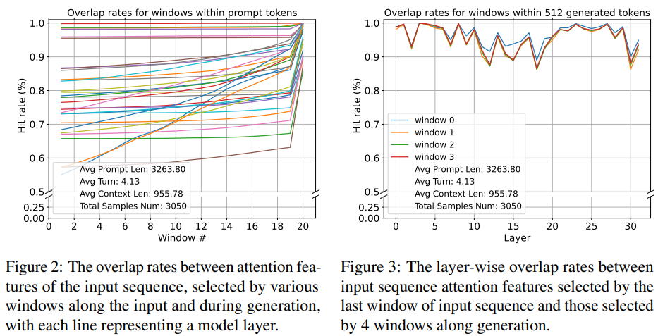
In order to verify the observation windows did reflects the attention distribution during the generation/decoding, the authors introduce hit rate as following.

Hit Rate: define a threshold $\theta$, during decoding/generation, denote important features as attention feature above theta. Hit rate is defined as following:

\[\begin{aligned} M_{\text{vote\_obs}} &= \operatorname{zeros\_like}\!\bigl(\mathbf{A}_{\text{cur}}\bigr) \\ M_{\text{vote\_obs}}[I] &= 1 \\ M_{\text{threshold\_cur}} &= \mathbf{1}\!\bigl(\mathbf{A}_{\text{cur}} > \theta\bigr) \\ \mathbf{O} &= M_{\text{threshold\_cur}} \wedge M_{\text{vote\_obs}} \\ H &= \frac{\sum \mathbf{O}}{\sum M_{\text{threshold\_cur}}} \end{aligned}\]

Step 1 here is to generate a all zero matrix from $\mathbb{R}^{N\times L_{\mathrm{prefix}}}$, which is the same size as $\mathbf{A}_{\text{cur}}$. Here $\mathbf{A}_{\text{cur}}$ represents attention feature between the current generated Q and the prefix K.

Step 2 and 3 is to make the corresponding position to be 1.

Finally to compute the overlapping rate between important feature during decoding/generation and the voting result (topK) from observation windows.

The following figure 2 showcased that the last window has the highest important feature overlapping rate for generation; figure 3 demonstrated, from layer perspective, tokens from generation still have the highest overlapping rate to the observation window, and this pattern is consistent (as generation goes on).

Pseudo code

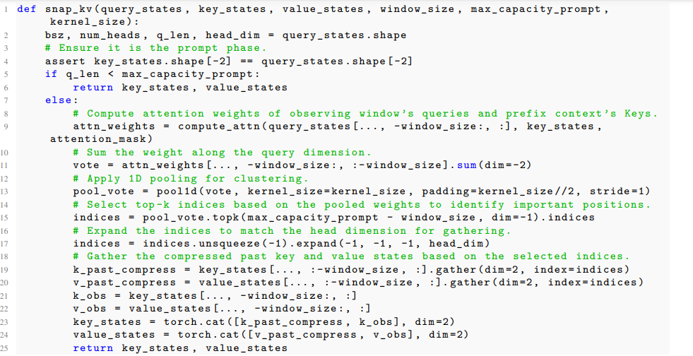
Here line 8-17 is for voting, line 18-24 is for actual compressing.

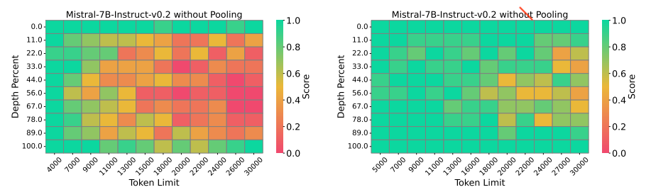
Worth to notice that here the author did not do a simple top-K directly, rather after a pooling (1-d conv) then top-K. A needle in hay stack experiment supports this idea

Final note on SnapKV

SnapKV validates an observation which is a consensus now: The important attention features change with different instructions, but it is irrelevant to the position of the instruction. In other words, if the prompt is composed by some context and instruction/question, the order does not matter, as the last observation window knows what to pay attention to.

SnapKV is a dynamic method (static method is with constant weighted importance, or fixed policy, like TurboQuant), namely at every inference, extra computation is needed using the last observation window’s attention to select token.

PyramidKV

Last work we will review for KV compression is PyramidKV which is a follow-up of SnapKV.

The main motivations/ideas:

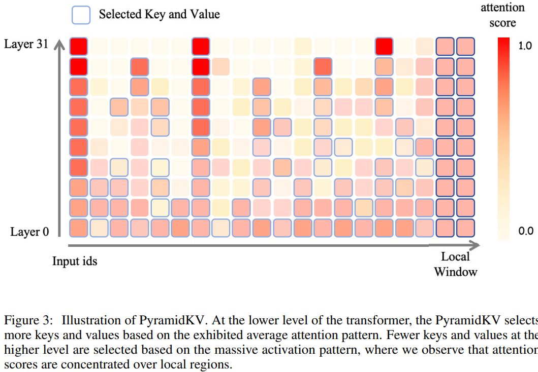
1. This approach dynamically adjust KV cache size across different layers
2. Allocate more cache in lower layers, and less in higher ones.
3. They are inspired by retrieval head study which discovered that upper layers has more ‘Massive activation’. Here massive activation means attention concentrates overwhelmingly on a few key tokens.

The authors identify a notable transition of attention distribution from a broad coverage of global contexts to a narrow focus of local tokens over layers in LLM. Namely, as the layer goes higher, the attention becomes more focused.

Algorithm in detail

1. One overall budget for KV cache:

   \[k^{\mathrm{total}} = \sum_{l=0}^{m-1} k^{l}\]

2. First allocate budgets to the first and the last layer as $k^{0} = \frac{2\,k^{\mathrm{total}}}{m},\ k^{m-1} = \frac{k^{\mathrm{total}}}{\beta\, m} - k^{0}$, respectively.

3. Then the middle layers can be configured as

   \[k^{l} = k^{m-1} - \frac{k^{m-1} - k^{0}}{m}\, l\]

4. Then the rest is the same as SnapKV: every layer keeps the top-$k^l$ tokens with pooling. One thing different from SnapKV is to keep all the KV for the observation window.

This selection mechanism can be viewed in the following figure.

Both SnapKV and PyramidKV did experiments on benchmark like HotpotQA, wiki, LCC, etc, with reasonable accuracy degraded and with only 50% (or even up to 12%) KV cache. They have similar affect as long-term memory, context compressing in agentic era.

KV quantization

Different from the (dynamic) compression algorithms, in this section we review a static way for KV ‘compression’ [5]: no selection of the token info, but save the storage for KV cache of each token.

Formally, a quantizer (quantization map) is denoted as $Q : \mathbb{R}^{d} \to {0,1}^{B}$. If $B = b\cdot d$ for a positive integer $b$, this quantizer will have a bit-width of $b$. This means $b$ bits are used to encode each coordination of a vector from $\mathbb{R}^{d}.$ The inverse mapping, dequantizer, is defined as $Q^{-1} : {0,1}^{B} \to \mathbb{R}^{d}$, which is lossy.

Notations: denote unit hypersphere in $\mathbb{R}^d$ as $\mathbb{S}^{d-1}$.

Quantization for unit vectors

In this section, we focus on the question about how to quantize unit, random vectors.

Foundation: unit random vector

The most important foundation of TurboQuant is the distribution of each coordination of the high-dimensional unit random vectors can be formulated analytically.

Lemma 1. For any positive integer $d$, if $x \in \mathbb{S}^{d-1}$ is a random variable uniformly distributed over the unit hypersphere, then for any $j \in [d]$ the coordinate $x_j$ follows the following (scaled/shifted, not dependent on $j$, only on $d$) Beta distribution:

\[x_j \sim f_X(x) \;:=\; \frac{\Gamma(d/2)}{\sqrt{\pi}\,\Gamma\bigl((d-1)/2\bigr)}\,(1 - x^2)^{(d-3)/2}. \]

In high dimensions this Beta distribution converges to the normal distribution $f_X(\cdot) \to \mathcal{N}(0,\,1/d)$.

Given this foundation 1, we can start to quantize a vector $x \in \mathbb{S}^{d-1}$. In order to make it a random vector, a random rotation matrix $\mathbf{\Pi} \in \mathbb{R}^{d \times d}$ is employed to randomize the vector as $\mathbf{\Pi} x \in \mathbb{S}^{d-1}$.

This paper is proposing a family random quantizers as solution, which needs the following 2 ways to measure the accuracy of this family: let $Q$ be a family of random quantizer, there are 2 distortion measures for any (worst-case) vectors $x,y\in\mathbb{R}^d$

\[\begin{aligned} \text{(MSE)} \quad D_{\mathrm{mse}} &:= \mathbb{E}_{Q}\!\left[ \left\| \mathbf{x} - Q^{-1}\bigl(Q(\mathbf{x})\bigr) \right\|_{2}^{2} \right] \\[0.4em] \text{(inner-prod error)} \quad D_{\mathrm{prod}} &:= \mathbb{E}_{Q}\!\left[ \left| \langle \mathbf{y}, \mathbf{x} \rangle - \langle \mathbf{y}, Q^{-1}\bigl(Q(\mathbf{x})\bigr) \rangle \right|^{2} \right] \end{aligned}\]

where the expectation is taken wrt all the quantizer in this family. One extra requirement for unbiasedness is defined as

\[\text{(unbiased inner-prod)} \quad\mathbb{E}_{Q}\bigl[ \langle \boldsymbol{y},\, Q^{-1}(Q(\boldsymbol{x})) \rangle \bigr]= \langle \boldsymbol{y},\, \boldsymbol{x} \rangle.\]

Note that the authors stated in Section 1.1 that ‘aim to design quantizer which minimize the measures’, the result here is not in strict optimal manner (not e.g., $\arg\min$), except for 1-D case, rather proved that for TurboQuant, the upper bound is pretty close to the theoretical lower bound.

In the following two subsection, we will look closer at 2 proposed family quantizers $\mathrm{TurboQuant}_\mathrm{mse}$ and $\mathrm{TurboQuant}_\mathrm{prod}$.

Near MSE optimal TurboQuant

Let us continue with the rotated vector $\mathbf{\Pi} x$ , by Lemma 1, we know that each coordination of it follows a Beta distribution. And for high dimension, these coordinates become nearly independent. Hence, the task to quantize $\mathbf{\Pi} x$ reduces to quantize each coordinate using a scalar quantizer, and this scalar random variable has density function

\[f_X(x) \;=\; \frac{\Gamma(d/2)}{\sqrt{\pi}\,\Gamma\bigl((d-1)/2\bigr)}\,(1 - x^2)^{(d-3)/2}, \mathrm{where} \ \ x\in [-1,1]\]

For scalar case, the (MSE) objective function can be formulated as

\[\mathcal{C}(f_X, b):= \min_{-1 \le c_1 \le c_2 \le \cdots \le c_{2^b} \le 1}\sum_{i=1}^{2^b}\int_{\frac{c_{i-1}+c_i}{2}}^{\frac{c_i+c_{i+1}}{2}}|x - c_i|^{2}\, f_X(x)\, dx .\]

This is because the expectation wrt $Q$ in (MSE) is equivalent to expectation wrt to rotation matrix ( $\mathbf{\Pi} x$ ), and for each coordination, it is just expectation over $[-1, 1]$. The problem above can be solved using numerical methods to achieve any precision. And it can be solved for different $b$ (say 1,2,3,4), and save the quantization map (centriods $c_i$’s) as codebook.

Now given this quantization for the scalar, the quantization of $\mathbf{\Pi} x$ is applied to each coordination, and the quantized value is the nearest centroid. The algorithm can be formulated as

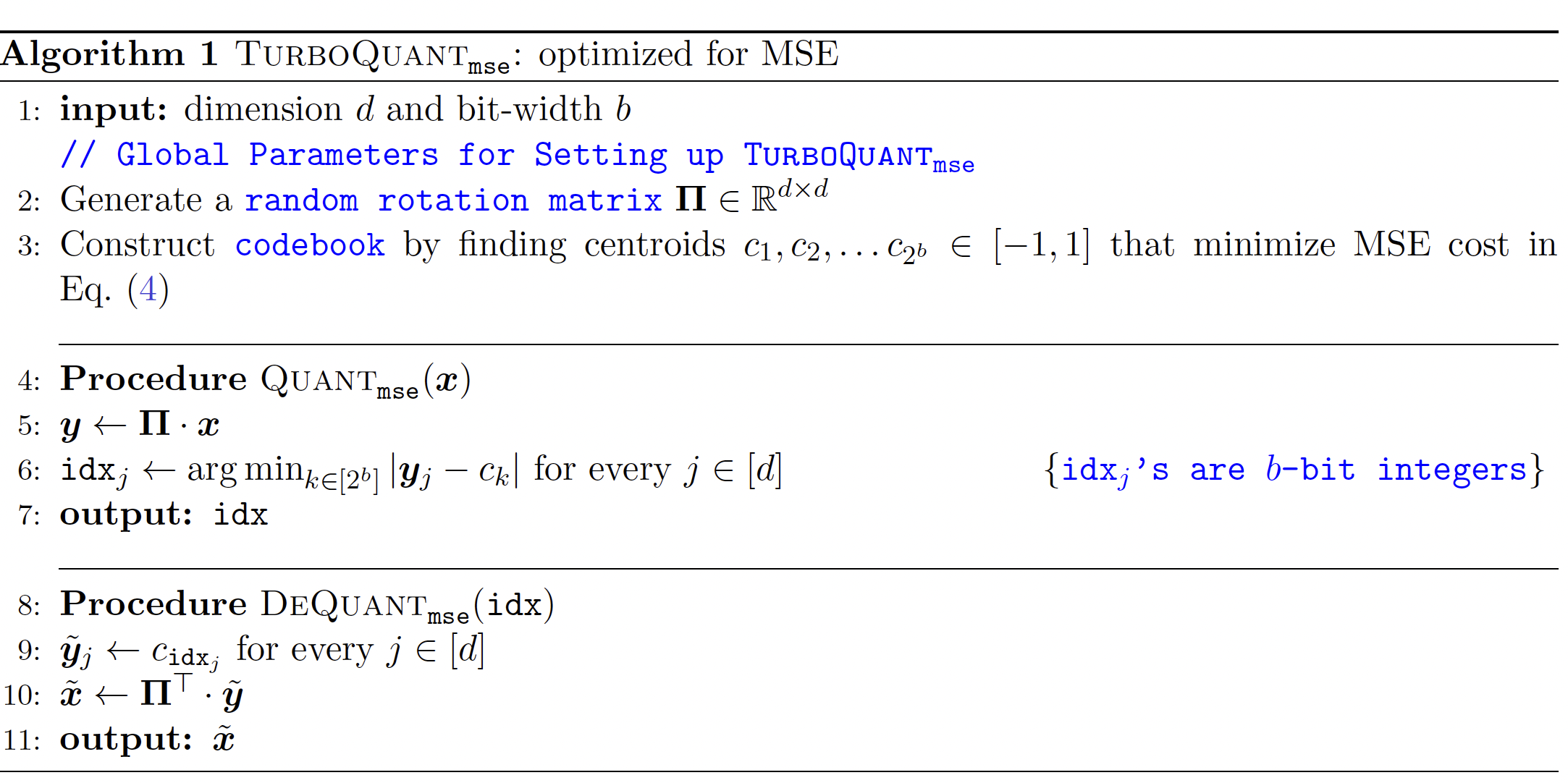
Now an important question is: what is the upper bound $D_{\mathrm{mse}}$ of the Algorithm 1. Theorem 1 in [5] proved that $D_{\mathrm{mse}}$ is bounded by $D_{\mathrm{mse}} \leq \frac{\sqrt{3\pi}}{2} \cdot \frac{1}{4^{b}}$. Note that this upper bound is independent wrt the vector dimension $d$. But there is hidden assumption of this paper which is $d$ should be large enough (coordinates become nearly independent for high dimensions). This is satisfied with modern KV cache vectors.

Why $D_{\mathrm{mse}} = \mathbb{E}\Bigl[ \bigl| \boldsymbol{y} - \tilde{\boldsymbol{y}} \bigr|_{2}^{2} \Bigr]$ ?

In the proof of Theorem, the first equality is actually very crucial. Due to the property of rotation matrix, we have $|\boldsymbol{x} - \tilde{\boldsymbol{x}}|_2 = |\boldsymbol{\Pi} \cdot \boldsymbol{x} - \tilde{\boldsymbol{y}}|_2 = |\boldsymbol{y} - \tilde{\boldsymbol{y}}|_2$ , hence

\[\begin{aligned} D_{\text{mse}} &= \mathbb{E}_Q[\|\boldsymbol{\Pi} \cdot \boldsymbol{x} - \tilde{\boldsymbol{y}}\|_2^2] \\ &= \mathbb{E}_{\boldsymbol{\Pi}}[\|\boldsymbol{\Pi} \cdot \boldsymbol{x} - \tilde{\boldsymbol{y}}\|_2^2] \\ & = \mathbb{E}_{\boldsymbol{\Pi}}[\|\boldsymbol{y} - \tilde{\boldsymbol{y}}\|_2^2] \end{aligned}\]

Then since this is for the worst-case vector $\boldsymbol{x}$, the expectation wrt $\boldsymbol{\Pi}$ is the same as the expectation to $\boldsymbol{y}$.

(Near) Inner-product Optimal TurboQuant

Since the Algorithm 1 (MSE TurboQuant) does not satisfy unbiased inner-prod, the author propose further Algorithm 2 (Inner-product Optimal TurboQuant)

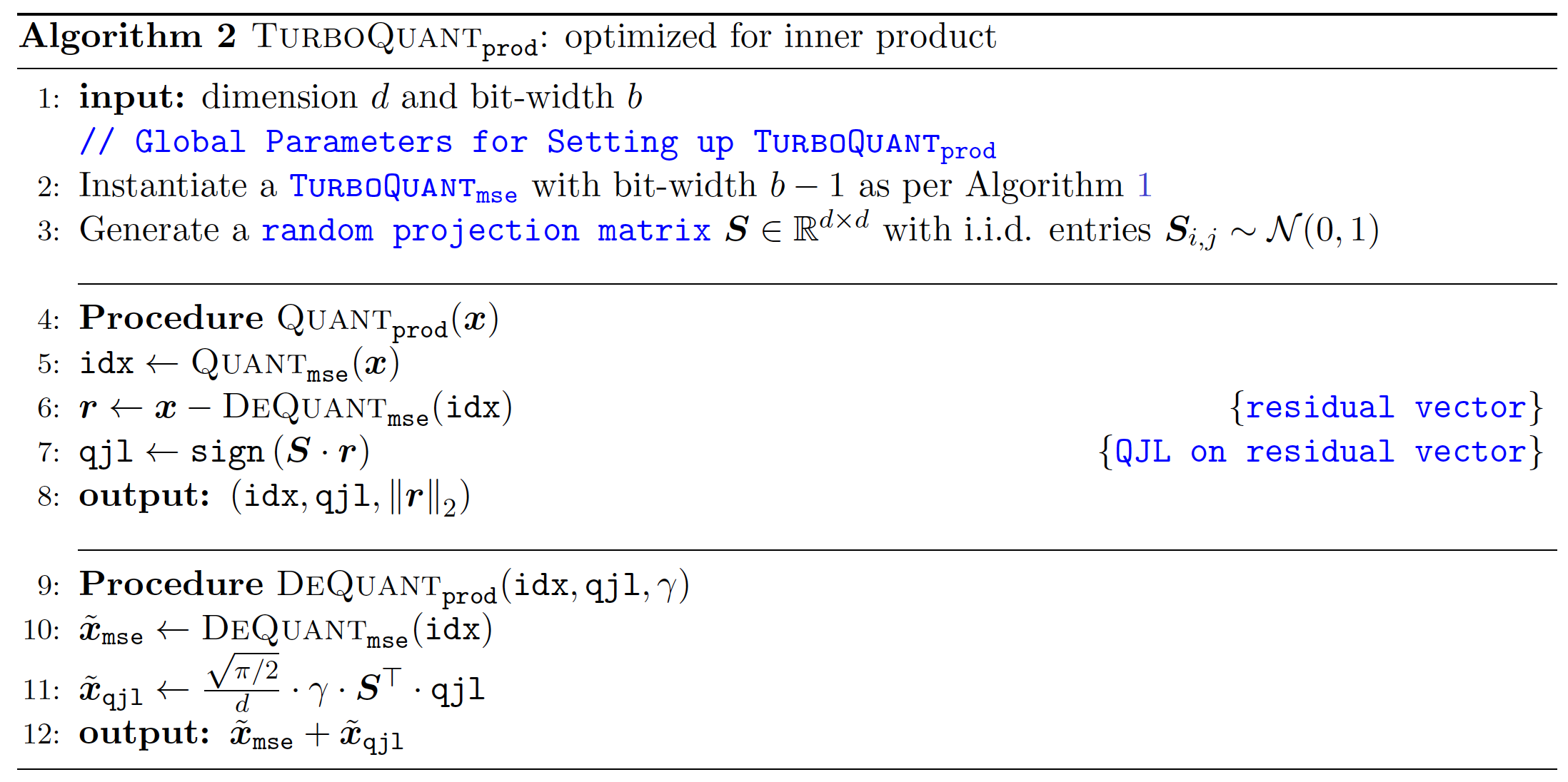
which applies QJL quantization on the residual wrt MSE TurboQuant.

The main result in this section (Theorem 2) proved that the expected inner product is unbiased, and provide the distortion upper bound $\frac{\sqrt{3}\,\pi^{2}\,\lVert \mathbf{y} \rVert_{2}^{2}}{d}\cdot\frac{1}{4^{b}}.$

Lower bounds

The authors also provided lower bound using Shannon Lower Bound lemma. These lower bounds means there are some worst case vector, such that the distortions are above those lower bounds.

For MSE TurboQuant, the lower bound is

\[D_{\mathrm{mse}}(Q) := \mathbb{E}\!\left[ \bigl\| \boldsymbol{x} - Q^{-1}\bigl(Q(\boldsymbol{x})\bigr) \bigr\|_{2}^{2} \right] \;\ge\; \frac{1}{4^{b}} .\]

and for inner-prod TurboQuant, it is

\[D_{\mathrm{prod}}(Q) = \mathbb{E}\!\left[ \bigl| \langle \boldsymbol{y}, \boldsymbol{x} \rangle - \langle \boldsymbol{y},\, Q^{-1}\bigl(Q(\boldsymbol{x})\bigr) \rangle \bigr|^{2} \right] \;\ge\; \frac{1}{d}\cdot\frac{1}{4^{b}} .\]

The gap are actually really small. For example, for MSE case, the upper bound is $\frac{\sqrt{3\pi}}{2} \cdot \frac{1}{4^{b}}$, especially when b is reasonably large.

Stronger result from RaBitQ [6]

All the result above are expectations, it averages the performance of the quantizers in that family. But [5] did not provide any analysis on the concentration of the distortions, except Fig 1 from empirical experiments.

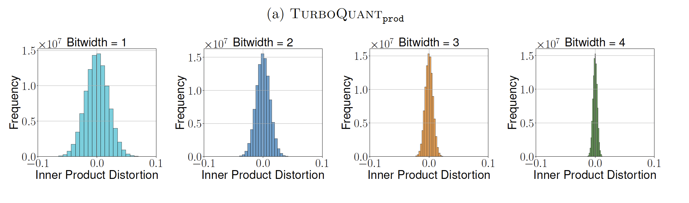
Theorem 3.2 in RaBitQ [6] proved that probability of the error of unbiased inner product quantizer $\mathrm{TurboQuant}_{\mathrm{prod}}$ being larger than

\[\sqrt{\frac{1 - \langle \bar{\mathbf{o}}, \mathbf{o} \rangle^{2}} {\langle \bar{\mathbf{o}}, \mathbf{o} \rangle^{2}}} \cdot \frac{\varepsilon_{0}}{\sqrt{D-1}}\]

is very small ( $2\, e^{-c_{0}\,\varepsilon_{0}^{2}}$ ), and the error will not deviate beyond $\mathcal{O}!\left(\frac{1}{\sqrt{D}}\right)$ with high probability.

TurboQuant on KV cache

For the KV quantization problem, only the keys need to keep the property of unbiased inner product, hence only keys are quantized using TurboQuant. The values are just weighted in the calculation of attention weights, hence it can be quantized with more coarse methods. The workflow now becomes as the following:

1. Given each key vector, normalize it to an unit vector, save the norm
2. Fix the target bit-width, apply Algorithm 2 to the unit vector with a prefixed random rotation matrix and projection matrix
3. Save the norm and corresponding state of each coordination (idx, qjl, and $\gamma$)
4. When calculate the attention later, de-quantization the key vector, and do normal multiplication with query vectors.

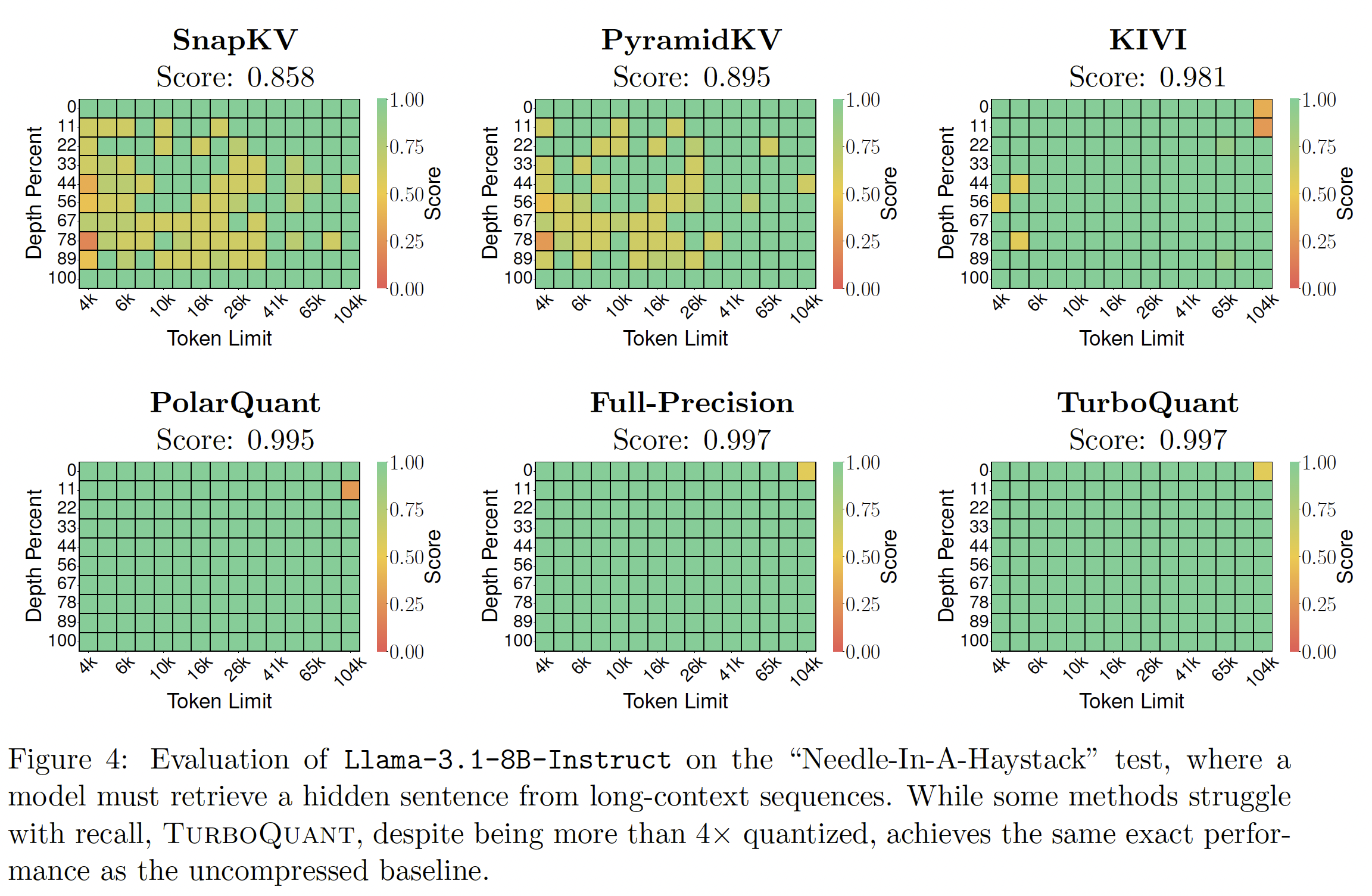
The author did the following needle-in-a-haystack test for the following KV compression/quantization method. And the performance of TurboQuant is impressive, although the result of SnapKV seems to be the one without pooling (different model, but similar size).

Concluding

As more and more AI agents deployed, the balance between the performance and token efficiency is crucial. Longer reasoning, more tool-calls, etc, the token dependence of the LLM will not be weakened. In the above picture, one single query triggered 7.8M tokens even though there are multiple LLM calls. KV cache management, combining KV compression and quantization, has big potential to mitigate this pressure.

Reference

1. Z.Liu, Et al. Scissorhands: Exploiting the Persistence of Importance Hypothesis for LLM KV Cache Compression at Test Time. 2023
2. A. Gupta, Et al. Memory-efficient Transformers via Top-k Attention. 2021
3. Y. Li, Et al. SnapKV: LLM Knows What You are Looking for Before Generation, 2024
4. Z.Cai, Et al. PyramidKV: Dynamic KV Cache Compression based on Pyramidal Information Funneling, 2024
5. A. Zandieh, Et al. TurboQuant: Online Vector Quantization with Near-optimal Distortion Rate, 2025
6. J.Gao, Et al. RaBitQ: Quantizing High-Dimensional Vectors with a Theoretical Error Bound for Approximate Nearest Neighbor Search, 2024