RL fundamental-part 1

Here we collect some basics about RL, especially towards LLM use case.

Basics

Some key concepts

1. Main components: Agent, Env
2. Action: $a_t$
3. State (of env) $s_t$, Reward $r_t$ can be derived based on the state
4. Goal of the agent: maximize its cumulative reward, called return, by learning an optimal policy.

Next we look at each concepts in more details

States and observations

1. States $s$: a complete description of the state of the env.
2. Observation $o$: a partial description of a state.
3. The states can be fully observed vs partially observed.

Action Spaces

1. Definition: all valid actions in a given env.
2. the action can be discrete or continuous.

Policies

1. Definition: a policy is a rule used by an agent to decide what actions to take.
2. Deterministic policy: $a_t = \mu(s_t).$
3. Stochastic policy: $a_t \sim \pi(\cdot \mid s_t)$.
4. $\pi(a\mid s)$ is the probability of choosing action $a$ at state $s$.
5. Policy is the ‘brain’ of the agent. Often in literature, people mix ‘agent’ and ‘policy’.
6. A very common format for stochastic policies: parameterized policies, i.e., depend on a NN,

Stochastic policies

Most advanced policies are stochastic. Two most common types

1. Categorical policies: discrete action space.
2. Diagonal Gaussian Policies: continuous action space.

Two key computations are crucial for using and training stochastic policies:

1. sampling actions from the policy
2. computing log likelihoods of particular action, $\log \pi_\theta (a\mid s)$. (the logarithm of the probability of choosing a specific action under a given policy).

Some intuitions of log likelihoods of particular actions

1. In policy optimization, we want to increase the likelihood of good actions (those leading to higher rewards) and decrease the likelihood of bad actions (those leading to lower rewards).
   • If $\pi_\theta (a\mid s)$ is high, the action is very likely, so the log likelihood will be positive and large.
   • If $\pi_\theta (a\mid s)$ is low, the action is less likely, so the log likelihood will be negative or close to zero.

Notes for Diagonal Gaussian Policies

Multi-variable Gaussian distribution are characterized by: mean vector $\mu,$ covariance matrix $\Sigma$.

Diagonal Gaussian distribution is a special case where $\Sigma$ is diag, which can be represented by a vector.

Then how to represent $\mu$ and covar $\Sigma$?

• A diagonal Gaussian policy always has a NN that maps from state (or obs) to mean actions, $\mu_\theta(s).$
• For $\Sigma$, two ways:
  1. Use a single vec of log standard deviations, $\log \sigma$ ( $\sigma$ is the standard deviation, diag of $\Sigma$). Here $\log \sigma$ is not dependent on state $s$. $\log \sigma$ is an extra learnable parameter. (TRPO, PPO, etc).
  2. Use a NN mapping from states $s$ to $\log\sigma_\theta (s).$ Here the NN can share some middle layer with $\mu_\theta(s).$

Note that in both cases we output log standard deviations instead of standard deviations directly. This is because log stds are free to take on any values in $(-\infty, \infty)$, while stds must be nonnegative. It’s easier to train parameters if you don’t have to enforce those kinds of constraints. 

Sampling

Given the mean action $\mu_\theta(s)$ and standard deviation $\sigma_\theta(s),$ and a vector $z\sim \mathcal{N}(0, I)$, an action sample can be computed with

The log-likelihood of a k-dim action a, with mean $\mu = \mu_\theta(s)$ and std $\sigma = \sigma_\theta(s),$ is

Trajectories

A trajectory $\tau$ is a sequence

$\tau = (s_0, a_0, s_1, a_1, …)$

The very first state $s_0\sim \rho_0(\cdot).$

The transitions can be deterministic or stochastic, $s_{t+1} = f(s_t, a_t),$ or $s_{t+1}\sim P(\cdot \mid s_t, a_t).$

Return and reward

Two critical concept to RL.

which can be simplified as $r_t = R(s_t),$ or $r_t = R(s_t, a_t).$ Given a trajectory $\tau$, two types of return:

1. Finite-horizon un-discounted return,

1. Infinite-horizon discounted return.

In RL real-life practice, it is frequent to set up algorithms to optimize the un-discounted return, but use discount factors in estimating value functions.

The RL Problem

Now we can formulate the classic RL problem. The probability of a T-step trajectory is ( $\tau$ ):

The expected return is :

where the integral is taken over all trajectories.

The central problem of RL

where $\pi^*$ is the optimal policy, i.e., to find the optimal policy which maximize the expected return.

Value function (==Expected return)

One problem of expected return in the previous section is that it can not be computed precisely (transition probability unknown, infinite trajectory etc).

Value: the expected return if you start in that state or state-action pair, and then act according to a particular policy forever after.

There are mainly 4 types of value functions:

1. On-policy Value Function, which gives the expected return if you start in state s and use policy $\pi$ forever

1. On-policy Action-Value Function, which gives the expected return if you start in state s, take an arbitrary action a (not necessarily sampled from the policy), and follow the policy $\pi$ forever

1. Optimal Value Function, which gives the expected return if you start in state  and always act according to the optimal policy in the environment:

1. Optimal action-value Function, which gives the expected return if you start in state s, take an arbitrary action a , and then forever act according to the optimal policy

Two simple conclusion:

and

The optimal Q func $Q^*(s,a)$ and the optimal Action

By definition, $Q^*(s,a)$ gives the expected return for starting state s, taking arbitrary action a, then following the optimal policy forever.

Then the optimal policy in s will be: select whichever action maximizes the expected return from starting in s. In other words， if we know $Q^(s,a)$, we can directly obtain the optimal action $a^(s)$

Bellman Equations

All four types of the value functions obey Bellman equation.

Intuition of Bellman: The value of your starting point is the reward you expect to get from being there, plus the value of wherever you land next.

Bellman eq for the on-policy value func:

where $s’\sim P$ means $s’\sim P(\cdot \mid s, a)$, and $a’\sim \pi(\cdot\mid s’)$.

Bellman eq for the optimal value func:

The main difference between these two types of Bellman func is with or without max. When there is max, whenever the agent gets to choose its action, in order to act optimally, it must choose action leads to the highest value.

Advantage Functions

This is to describe how much better an action is than others on average

which describes how much better it is to take a specific action a  in state s, over randomly selecting an action according to $\pi(\cdot\mid s)$, assuming you act according to forever after. 

Types of RL algorithms

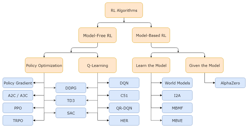
We mainly focus on model-free RL. Model-based RL algorithm includes world models, dreamers etc. For model free RL, there are mainly two approaches.

Two main approaches

Policy optimization

Methods in this family represent a policy as $\pi_\theta (a\mid s)$. They optimize the parameters $\theta$ by either

• directly by gradient ascent on the performance obj $J(\pi_\theta)$

• or indirectly, by maximizing local approximation of $J(\pi_\theta).$

This optimization is always performed on-policy, which means that each update only uses data collected while acting according to the most recent version of the policy.

Policy optimization also usually involves learning an approximator $V_\phi(s)$ for the on-policy value function $V^\pi(s)$, which gets used in figuring out how to update the policy.

and

1. A2C/A3C: direct gradient ascent to maximize performance.
2. PPO: whose updates indirectly maximize performance, by instead maximizing a surrogate objective function, which gives a conservative estimate for how much $J(\pi_\theta)$ will change as a result of the update.

Q-learning

Learn an approximator $Q_\theta(s,a)$ for the optimal action-value function, $Q^*(s,a).$

It is usually Off-policy, which means that each update can use data collected at any point during training, regardless of how the agent was choosing to explore the environment when the data was obtained (no constrains from policy).

In other words, in Q-learning, the data (s,a,r,s′,done) is stored in replay buffer, which can be reused.

The action taken by the Q-learning agent is given by

Some known algorithm includes DQN, C51 etc.

Of course, mixture

• DDPG: an algorithm which concurrently learns a deterministic policy and a Q-function by using each to improve the other,
• SAC: a variant which uses stochastic policies, entropy regularization, and a few other tricks to stabilize learning and score higher than DDPG on standard benchmarks.

In this scenario, we have

1. Actor — Learns the policy $\pi_\theta$ and decides actions.
2. Critic — Evaluates the value function (V(s), expected return) to guide the actor.

In the remaining part of this note, we review some classic algorithms.

Policy optimizations

Here we discuss the mathematical foundations of policy optimization algorithms.

Simplest policy gradients

Objective: find a stochastic policy $\pi_\theta$, which maximize expected return $J(\pi_\theta) = E_{\tau \sim \pi_\theta}[R(\tau)]$. We consider finite-horizon undiscounted return.

A straightforward way is using gradient ascent

The term $\nabla_\theta J(\pi_\theta)$ is called the policy gradient.

We need to lay out some facts.

1. Probability of a traj $\tau = (s_0, a_0, …, s_{T+1})$ is that

1. Log-derivative trick.

1. Grad-log-prob of a traj.

So, we derive that

This is an expectation, which means we can estimate it with a sample mean：

where $\mathcal{D} = {\tau_i}{i=1, …, N}$ are the trajectories by letting the agent act in the env using the policy $\pi\theta$. This is the simplest version of the computable expression of policy gradient.

Code implementation

1. making the policy network

# make core of policy network
logits_net = mlp(sizes=[obs_dim]+hidden_sizes+[n_acts])

# make function to compute action distribution
def get_policy(obs):
    logits = logits_net(obs) # logits means the probility is from a softmax func.
    return Categorical(logits=logits)

# make action selection function (outputs int actions, sampled from policy)
def get_action(obs):
    return get_policy(obs).sample().item()

Categorical object is a PyTorch Distribution object that wraps up some mathematical functions associated with prob distributions.

2. Making the loss function

# make loss function whose gradient, for the right data, is policy gradient
def compute_loss(obs, act, weights):
    logp = get_policy(obs).log_prob(act)
    return -(logp * weights).mean()

get_policy(obs).log_prob(act) = $\log \pi_\theta(a_t \mid s_t)$.

weights is reward or advantage, i.e., $R(\tau)$. Weight for a state-action pair is the return from the episode to which it belongs.

what is right data? A set of (state, action, weight) tuples collected while acting according to the current policy, i.e., samples.

Note on this loss function

Here the loss function is not a loss function in the sense of supervised learning.

1. t传统的损失函数中，数据分布(features, labels)通常是固定的，并且独立于我们要优化的参数。而在强化学习中，数据是从当前的策略中采样的，因此数据分布依赖于参数 (state, action, rewards)。也就是说，策略的更新会影响数据的分布，这与传统的损失函数不同。 2.
   • 传统的损失函数通常衡量我们关心的性能指标。在监督学习中，损失函数可以评估模型的误差，通常与我们希望优化的目标（如准确率、损失值等）直接相关。但在这里，我们关心的是 期望回报 $J(\pi_\theta)$，而这个“损失函数”并没有直接近似这个回报，甚至在期望上也没有直接关系。它之所以对我们有用，仅仅是因为当我们使用当前参数和当前策略生成的数据来评估这个“损失函数”时，它的梯度就是期望回报的负梯度。
   • 但是，在第一次梯度下降步骤之后，这个“损失函数”就与性能没有什么关系了。也就是说，最小化这个“损失函数”并不意味着期望回报会提高。对于给定的一个数据批次，这个损失函数没有任何保证能够提升期望回报。你可以把这个损失函数最小化到负无穷大，但策略的表现可能会变得更差，实际上通常会发生这种情况。深度强化学习研究人员有时会形容这种情况为“策略过拟合于一个数据批次”，但是这种说法是描述性的，不能字面理解，因为它并不指代传统意义上的泛化误差。

3. running for one epoch

# for training policy
def train_one_epoch():
    # make some empty lists for logging.
    batch_obs = []          # for observations
    batch_acts = []         # for actions
    batch_weights = []      # for R(tau) weighting in policy gradient
    batch_rets = []         # for measuring episode returns
    batch_lens = []         # for measuring episode lengths

    # reset episode-specific variables
    obs = env.reset()       # first obs comes from starting distribution
    done = False            # signal from environment that episode is over
    ep_rews = []            # list for rewards accrued throughout ep

    # render first episode of each epoch
    finished_rendering_this_epoch = False

    # collect experience by acting in the environment with current policy
    while True:

        # rendering
        if (not finished_rendering_this_epoch) and render:
            env.render()

        # save obs
        batch_obs.append(obs.copy())

        # act in the environment
        act = get_action(torch.as_tensor(obs, dtype=torch.float32))
        obs, rew, done, _ = env.step(act)

        # save action, reward
        batch_acts.append(act)
        ep_rews.append(rew)

        if done:
            # if episode is over, record info about episode
            ep_ret, ep_len = sum(ep_rews), len(ep_rews)
            batch_rets.append(ep_ret)
            batch_lens.append(ep_len)

            # the weight for each logprob(a|s) is R(tau)
            batch_weights += [ep_ret] * ep_len

            # reset episode-specific variables
            obs, done, ep_rews = env.reset(), False, []

            # won't render again this epoch
            finished_rendering_this_epoch = True

            # end experience loop if we have enough of it
            if len(batch_obs) > batch_size:
                break

    # take a single policy gradient update step
    optimizer.zero_grad()
    batch_loss = compute_loss(obs=torch.as_tensor(batch_obs, dtype=torch.float32),
                              act=torch.as_tensor(batch_acts, dtype=torch.int32),
                              weights=torch.as_tensor(batch_weights, dtype=torch.float32)
                              )
    batch_loss.backward()
    optimizer.step()
    return batch_loss, batch_rets, batch_lens

1. Here one episode ran in if done loop,
2. Then the optimizer.zero_grad(), batch_loss.backward() and optimizer.step() . Especially, batch_loss.backward() connect to the policy network logits_net via compute_loss function.

Expected grad-log-prob lemma

Lemma: Suppose that $P_\theta$ is a parameterized probability distribution over a random variable $x$, then

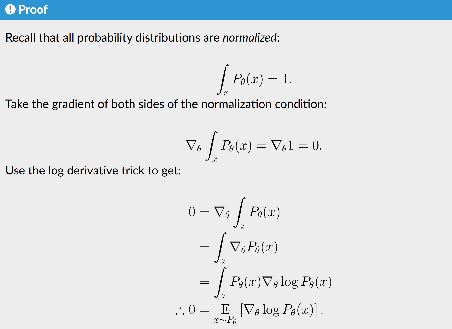
Don’t let the past distract you

Based on the grad-log-prob lemma, we can further simplify the policy gradient

This is because the term $t’<t$ are constant and the previous lemma says the expectation is zero.

The term

is called reward-to-go.

Implementation Reward-to-go

def reward_to_go(rews):
    n = len(rews)
    rtgs = np.zeros_like(rews)
    for i in reversed(range(n)):
        rtgs[i] = rews[i] + (rtgs[i+1] if i+1 < n else 0)
    return rtgs

Then modify

                # the weight for each logprob(a|s) is R(tau)
                batch_weights += [ep_ret] * ep_len

to

                # the weight for each logprob(a_t|s_t) is reward-to-go from t
                batch_weights += list(reward_to_go(ep_rews))

Baselines in Policy gradients

EGLP Lemma can be rewritten as

And an immediate consequence can be, for any function of $s_t$, we have

This allows us to manipulate the policy gradient as

Any function $b$ used in this way is called a baseline.

Note on baseline

The most common choice of baseline is the on-policy value function $V^\pi(s_t)$. Recall that this is the average return an agent gets if it starts in state $s_t$ and then acts according to policy $\pi$ for the rest of its life.

Empirically, the choice

has the desirable effect of reducing variance in the sample estimate for the policy gradient. This results in faster and more stable policy learning. It is also appealing from a conceptual angle: it encodes the intuition that if an agent gets what it expected, it should “feel” neutral about it.

In practice, $V^\pi(s_t)$ can not be computed exactly, so it has to be approximated, usually done with a Neural Network $V_\phi (s_t)$. This NN is concurrently updated with the policy.

The simplest method for learning $V_\phi (s_t)$, (used in TRPO, PPO, A2C), is to minimize the obj

where $\pi_k$ is the policy at epoch $k$. This is done with one or more steps of gradient descent, starting from the previous value parameters $\phi_{k-1}$.

Other forms of the policy gradient.

The policy gradient has the general form

where $\Phi_t$ could be any of $R(\tau)$, or $\sum_{t’=t}^T R(s_{t’}, a_{t’}, s_{t’+1})$, or $\sum_{t’=t}^T R(s_{t’}, a_{t’}, s_{t’+1})-b(s_t)$.

We could have two more choices.

1. On-policy Action-value function.

   \[\Phi_t = Q^{\pi_\theta} (s_t, a_t).\]

2. The advantage function.

Alg 1: vanilla policy gradient (VPG)

Quick facts

• VPG is an on-policy algorithm.
• VPG can be used for environments with either discrete or continuous action spaces.

Key equations

Let $\pi_\theta$ denote a policy with parameters $\theta$, and $J(\pi_\theta)$ denote the expected finite-horizon undiscounted return of the policy. The gradient of $J(\pi_\theta)$ is

where $A^{\pi_\theta}$ is the advantage function for the current policy.

Update the policy as usual

Exploration vs Exploitation

VPG trains a stochastic policy in an on-policy way. This means that it explores by sampling actions according to the latest version of its stochastic policy. The amount of randomness in action selection depends on both initial conditions and the training procedure. Over the course of training, the policy typically becomes progressively less random, as the update rule encourages it to exploit rewards that it has already found. This may cause the policy to get trapped in local optima.

Pseudocode

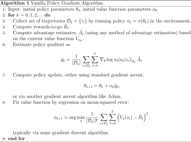
Here $\phi$ is NN for value function $V$, and $\theta$ for policy network.

Alg 2: TRPO

TRPO updates policies by taking the largest step possible to improve performance, while satisfying a special constraint on how close the new and old policies are allowed to be. The constraint is expressed in terms of KL-Divergence, a measure of distance between probability distributions.

This is different from normal policy gradient, which keeps new and old policies close in parameter space. But even seemingly small differences in parameter space can have very large differences in performance—so a single bad step can collapse the policy performance. This makes it dangerous to use large step sizes with vanilla policy gradients, thus hurting its sample efficiency. TRPO nicely avoids this kind of collapse, and tends to quickly and monotonically improve performance.

Quick facts

• TRPO is an on-policy algorithm.
• TRPO can be used for environments with either discrete or continuous action spaces.

Key equations

Let $\pi_\theta$ denote a policy with parameters $\theta$. The theoretical TRPO update is :

where $\mathcal{L}(\theta_k, \theta)$ is the surrogate advantage function, a measure of how policy $\pi_\theta$ performs relative to the old policy $\pi_{\theta_k}$ using data from the old policy:

And $\bar{D}_{KL}(\theta \Vert \theta_k)$ is an average KL-divergence between policies across states visited by the old policy:

Note

The objective and constraint are both zero when $\theta = \theta_k.$

Approximated implementation

The theoretical TRPO is not easy to work with, so TRPO makes some approximation (Taylor expand the obj and constraints)

The problem can be rewritten as

Using Lagrangian duality, we have the following analytic solution：

One problem with the above iteration is that, due to Taylor expansion error, this may not satisfy the KL constraint, or actually improve the surrogate advantage. So, a modified iteration is given as following:

where $\alpha \in (0,1)$ is the backtracking coefficient, and $j$ is the smallest nonnegative integer such that $\pi_{\theta_{k+1}}$ satisfies the KL constraint and produces a positive surrogate advantage.

Note

The gradient $g$ of the surrogate advantage function w.r.t. $\theta$, evaluated at $\theta = \theta_k$, is exactly equal to the policy gradient $\nabla_\theta J(\pi_\theta).$

Alg 3: PPO

Motivation

Same as TRPO, how can we take the biggest possible improvement step on a policy using the data we currently have, without stepping so far that we accidentally cause performance collapse?

Quick facts

PPO is a family of first-order methods.

PPO methods are significantly simpler to implement, and empirically seem to perform at least as well as TRPO.

• PPO is an on-policy algorithm.
• PPO can be used for environments with either discrete or continuous action spaces.

We focus on PPO-clip (one variant of PPO) in this note.

Key equations

PPO-clip updates policies via

Here $L$ is given by

The first term is the same as in TRPO, which is a measure of how policy $\pi_\theta$ performs relative to the old policy $\pi_{\theta_k}$ using data from the old policy.

The $\epsilon$ is a small hyperparam which roughly says how far away the new policy is allowed to go from the old.

A simpler version

where

Analysis of these two cases.

Advantage is positive

In this case the obj is

Since

advantage is positive means the obj L will increase if the action becomes more likely, in other words, if $\pi_\theta(a\mid s)$ increases. And the min in this term puts a ceiling on how much the obj can increase.

Advantage is negative

In this case, the obj becomes

Since the advantage is negative, the obj will increase if the action becomes less likely, in other words, if $\pi_\theta(a\mid s)$ decreases. $1-\epsilon$ part puts a ground.

Pseudocode

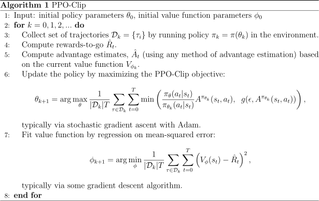
Here $\phi$ is NN for value function $V$, and $\theta$ for policy network.

Alg 4: DDPG

Deep Deterministic Policy Gradient (DDPG) is an algorithm which concurrently learns a Q-function and a policy.

• Q-func learning: uses off-policy data and the Bellman equation,
• policy learning: uses the Q-function to learn the policy.

Motivation

If you know the optimal action-value function $Q^*(s,a),$ then in any given state, the optimal action is

( $Q^*$ : if you start in state s, take an arbitrary action a , and then forever act according to the optimal policy).

DDPG interleaves learning an approximator to $Q^(s,a)$ with learning an approximator to $a^(s)$, and it does so in a way which is specifically adapted for env with continuous action space.

Difficulty: for continuous action space, compute $\max_a Q(s,a)$ is very expensive and difficult.

Quick facts

• DDPG is an off-policy algorithm.
• DDPG can only be used for environments with continuous action spaces.
• DDPG can be thought of as being deep Q-learning for continuous action spaces.

Key Equations

Mainly two parts, learning a Q function, learning a policy.

Q-learning

Recall Bellman equation which is the starting point for Q-learning

where $s’\sim P(\cdot\mid s,a).$

Suppose the approximator is a NN $Q_\phi(s,a)$, and that we have collected a set $\mathcal{D} = {(s,a,r,s’,d)}.$ Then we can set up a mean-squared-Bellman-error (MSBE) func

Here $d$ indicates whether $s’$ is terminal.

DDPG and DQN are largely based on minimize MSBE func. Two main tricks.

Trick 1: replay buffers

The set $\mathcal{D}$ of previous experiences is used as replay buffer.

In order for the algorithm to have stable behavior, the replay buffer should be large enough to contain a wide range of experiences, but it may not always be good to keep everything. If you only use the very-most recent data, you will overfit to that and things will break; if you use too much experience, you may slow down your learning.

We’ve mentioned that DDPG is an off-policy algorithm: this is as good a point as any to highlight why and how. Observe that the replay buffer should contain old experiences, even though they might have been obtained using an outdated policy. Why are we able to use these at all? The reason is that the Bellman equation doesn’t care which transition tuples are used, or how the actions were selected, or what happens after a given transition, because the optimal Q-function should satisfy the Bellman equation for all possible transitions. If Bellman equation is employed, the method is off-policy.

Trick 2: Target Networks

is called Target. Due to minimizing MSBE, we try to make $Q$ funciton —> the target. BUT, they depends on the same parameters $\phi$.

• In DQN, the target is just copied over from the main network every some-fixed-number of steps.
• In DDPG,

where $\rho\in(0,1)$ is the polyak parameter.

DDPG detail

As mentioned earlier: computing the maximum over actions in the target is a challenge in continuous action spaces. DDPG deals with this by using a target policy network to compute an action which approximately maximizes $Q_{\phi_{targ}}$. The target policy network is found the same way, by polyak averaging the policy parameters over the course of training.

Putting it all together, DDPG Q-learning is done by minimizing the following MSBE loss using SGD

where $\mu$ is the target policy.

Policy-learning

Policy learning in DDPG is simple.

Pseudocode

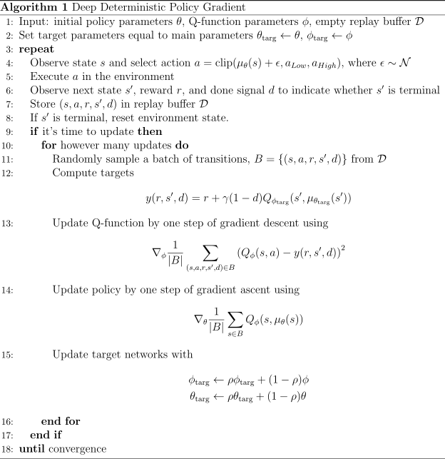
Alg 5: SAC

Soft Actor Critic (SAC) is an algorithm that optimizes a stochastic policy in an off-policy way, forming a bridge between stochastic policy optimization and DDPG-style approaches.

A central feature of SAC is entropy regularization. The policy is trained to maximize a trade-off between expected return and entropy, a measure of randomness in the policy. This has a close connection to the exploration-exploitation trade-off: increasing entropy results in more exploration, which can accelerate learning later on. It can also prevent the policy from prematurely converging to a bad local optimum.

Quick facts

• SAC is an off-policy algorithm.
• The version of SAC implemented here can only be used for environments with continuous action spaces.

Key equations

First, we introduce the entropy-regularized reinforcement learning setting.

Entropy-regularized reinforcement learning setting.

Entropy says how random a random variable is.

Let $x$ be a random variable with density func $P.$ The entropy $H$ of x is

Entropy-regularized RL is

where $\alpha>0$ is a trade-off coefficient.

SO, we have different value functions

and

These two are connected by

and the Bellman eq for $Q^\pi$ is

Soft Actor-critic

Actor critic meaning are defined in Kinds of RL alg.

Some details derivations are introduced in https://spinningup.openai.com/en/latest/algorithms/sac.html

Alg 6: GRPO

This method is firstly proposed by deepseek math paper https://arxiv.org/pdf/2402.03300 and this note is the whole paper, not only GRPO

Key findings

• The mathematical reasoning capability of DeepseekMath is attributed to two key factors:
  1. Good dataset: publicly available web data through a meticulously engineered data selection pipeline.
  2. GRPO enhances mathematical reasoning abilities. This method is a variant of PPO, but concurrently optimizing the memory usage of PPO.
• Created Deepseek-math Corpus, 120B math tokens. This preparation include further refine through human annotation.
• Deepseek-math Corpus is multilingual.
• DeepseekMath-base 7B is initialized with Deepseek-coder-base-v1.5 7B, as we notice that starting from a code training model is a better choice compared to a general LLM. (Should be true for SFT as well?)
• DeepseekMath-base 7B is trained with 500B tokens.
• Code training benefits math reasoning
• ArXiv paper seem Ineffective in improving math reasoning.
• Section 5.2.1 gives a unified paradigm (a unified equation)can incorporate the objective functions of SFT, RL (PPO, GRPO) .
• Why RL works? : RL enhances the model’s overall performance by rendering the output distribution more robust; in other words, it seems that the improvement is attributed to boosting the correct response from TopK rather than the enhancement of fundamental capabilities.
• Appendix contains the policy gradient formulation of GRPO.

SFT

Dataset: problems are paired with solutions in chain of thought, program of thought, and tool-integrated reasoning format.

Total number of training examples: 776K.

DeepSeekMath-instruct 7B undergoes mathematical instruction tuning based on DeepSeekMath-base.

Training examples are randomly concatenated until reaching a maximum context length of 4K token. ?? (This needs to be verified, using llama factory)

RL related findings

GRPO foregoes (放弃) the critic model (which estimate the value function V(s)), instead estimating the baseline from group scores, significantly reducing training resources. One fewer NN to train?

RL

Pretrain —> SFT —> RL has been proven to be effective in further improving the mathematical reasoning.

GRPO is a variant of PPO.

PPO is an actor-critic RL algorithm. (Actor: policy learning; critic: value function learning).

For LLM with PPO, it optimizes LLMs by maximizing the following surrogate objective:

where $\pi_\theta$ and $\pi_{\theta_{old}}$ are the current and old policy models, and $q,o$ are questions and outputs sampled from the question dataset and the old policy $\pi_{\theta_{old}}$, respectively. $\epsilon$ is a clipping hyperparameter for stabilizing training. $A_t$ is the advantage, which is estimated based on rewards ${r_{\geq t} }$ and a learned value function $V_{\varphi}$.

Thus, in PPO, a value function needs to be trained alongside the policy model and to mitigate over-optimization of the reward model, the standard approach is to add a per-token KL penalty from a reference model in the reward at each token, i.e.,

where $r_{\varphi}$ is the reward model, $\pi_{ref}$ is the reference model, which is usually the initial SFT model, and $\beta$ is the coefficient of the KL penalty.

Example

I want to do PPO (RLHF) toward llama-8b

1. Reward model: evaluates the quality of the generated text and provides feedback to the agent (policy model). The reward model is trained to predict human-provided feedback (e.g., a ranking or score given to a generated text) or other reward signals. For instance, if human raters score the quality of generated text on a scale (e.g., 1-5, or chosen/rejected), the reward model is trained to predict those scores based on the input-output pairs (context and generated text). A smaller model, such as a Llama-1B or a fine-tuned Llama-8B, can be used here. The reward model can be the same architecture as your base model (Llama-8B) but trained on a specific task (supervised learning on human feedback).
2. Policy model: The policy model is the one you’re actually optimizing in the RL setting. It generates text based on the input, and its goal is to maximize the reward signal it receives from the reward model. The policy model is typically a version of the trained LLM. The policy is essentially the “agent” that interacts with the environment (generating text), receiving feedback (from the reward model), and adjusting its behavior to improve over time.
3. Value model (value function): The value model estimates the expected future reward given a certain state (or context). It’s typically used in the actor-critic RL framework, where the actor is the policy model and the critic is the value model. The value model predicts the expected cumulative reward for a given input (state). The value model can be a smaller model, often a feedforward neural network or a lightweight version of your LLM.
4. Reference Model (or Behavior model): The reference model is typically a copy of the initial LLM. This model is not updated during the RL training.

How to understand the above LLM+PPO

1. Advantage: how much better an action is than others on average ( $V^\pi (s) = E_{a\sim \pi} [Q^\pi(s, a)]$ )

1. a measure of how policy $\pi_\theta$ performs relative to the old policy $\pi_{\theta_k}$ using data from the old policy:

An example of this surrogate objective is in Analysis of these two cases.

1. In practice, the reward model is usually a smaller LLM (or copy of your SFT LLM), trained on a dataset with ‘chosen’ and ‘rejected’ tags to add (human) preference.

For example:

{
        "conversations": [
            {
                "from": "human",
                "value": "There are 290 liters of oil in 24 cans. If 10 of the cans are holding 8 liters each, how much oil is each of the remaining cans holding?"
            }
        ],
        "chosen": {
            "from": "gpt",
            "value": "\n 1. We have 290 liters of oil in 24 cans.\n2. Out of these 24 cans, 10 cans are holding 8 liters each. Therefore, the total amount of oil in these 10 cans would be:\nTotal oil in 10 cans = Number of cans \\* Oil per can\n= 10 cans \\* 8 liters/can\n= 80 liters\n3. The remaining 14 cans must contain the rest of the oil. So, the total amount of oil in these 14 cans would be:\nTotal oil in 14 cans = Total oil - Total oil in 10 cans\n= 290 liters - 80 liters\n= 210 liters\n4. To find out how much oil is in each of the 14 cans, we divide the total oil in 14 cans by the number of cans:\nOil per can = Total oil in 14 cans / Number of cans\n= 210 liters / 14 cans\n≈ 15 liters/can\n\nTherefore, each of the remaining 14 cans is holding approximately 15 liters of oil."
        },
        "rejected": {
            "from": "gpt",
            "value": " 1. We know that there are 290 liters of oil in total and 10 of the cans hold 8 liters each. So we can calculate the amount of oil in those 10 cans as follows:\nOil in 10 cans = Total oil / Oil per can\n= 290 liters / 8 liters/can\n= 36.25 liters\n2. Now we need to find out how much oil is left in the other 14 cans. To do this, we subtract the amount of oil in the 10 cans from the total oil:\nRemaining oil = Total oil - Oil in 10 cans\n= 290 liters - 36.25 liters\n= 253.75 liters\n3. Finally, we divide the remaining oil by the number of cans to find out how much oil is in each of the remaining cans:\nOil per can = Remaining oil / Number of cans\n= 253.75 liters / 14 cans\n≈ 18.05 liters/can\n\nSo each of the remaining cans is holding approximately 18.05 liters of oil. \n"
        }
    },

1. The policy is about how LLM generate logits (distribution over vocab). Ref model is a copy of your SFT model, which will not be modified during training. Surrogate obj is trying to make sure each update is not so far from the previous step. Reward with KL divergence is to make sure the reward is not so far from the reward model, and the reference model.

Why PPO is not so good.

1. Value function in PPO is typically another model of comparable size of the policy model. More mem and computational burden.
2. Value function is treated as a baseline in the calculation of the advantage.
3. In the LLM context, usually only the last token is assigned a reward score by the reward model, this complicates the training of a value function that is accurate at each token. (value function is defined to predict reward for each token， but LLM usually only have reward for the last token (from reward model)).

GRPO

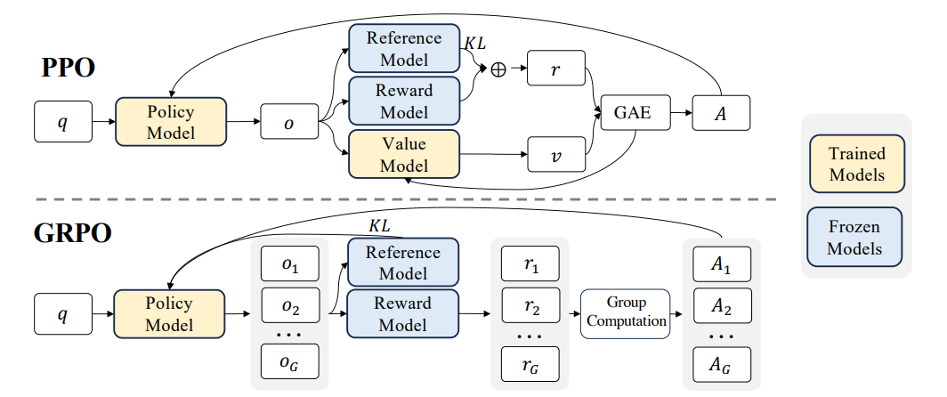
To obviate (消除) the need for additional value function approximation as in PPO, and instead uses the average reward of multiple sampled outputs, produced in response to the same question, as the baseline.

In other words, for each question $q$, GRPO samples a groups of outputs ${o_1, o_2, \ldots, o_G }$ from the old policy $\pi_{\theta_{old}}$ and then optimizes the policy model by maximizing the following obj

where $\hat{A}_{i,t}$ is the advantage calculated based on relative rewards of the outputs inside each group only. The group relative way that GRPO leverages to calculate the advantages, aligns well with the comparative nature of the reward models, as reward model are typically trained on datasets of comparisons between outputs on the same questions.

Also, instead of adding KL divergence in the reward, GRPO regularizes by directly adding the KL div between the trained policy and the reference policy to the loss.

After this reading, the following figure makes sense:

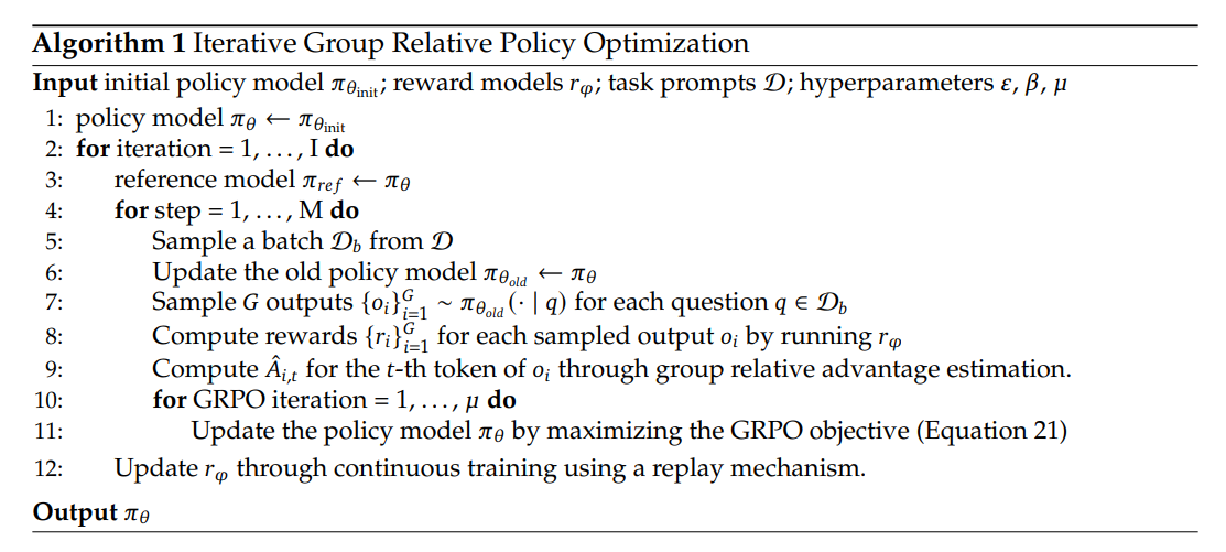
The pseudocode is given as

Note

1. Outcome supervision RL with GRPO (how to calculate advantage in a group)

Given a question $q$, a group of outputs ${ o_1, o_2, \ldots, o_G }$ are sampled from old policy model $\pi_{\theta_{old}}$. A reward model gives rewards, then $\hat{A}_{i,t} = \frac{r_i - mean(\mathbf{r})}{std(\mathbf{r})}$.

1. As RL training process progresses, the old reward model may not be sufficient to supervise the current policy model. So there is the iterative RL with GRPO in the psudocode line 12.

RLHF

This is more like framework, not constrained to any specific RL algorithms, even thought mainly used methods are PPO and GRPO.

It for each query, the initial LLM generates say 5 responses, and human labelers are asked to rank the responses.

Upside

1. We can run RL in arbitrary domain.
2. It is easier for human to discriminate than to generate. e.g., “write a poem” vs “which of these 5 poems is the best?”

Downside

1. We use human labelled data to train the reward model. The reward model can have billions parameters. It is very likely that the reward model can get a high score with some nonsense response. In other words, the env that RL is playing against is very complex and far more subtle than the one represented by the human labelled data. So, RL can discover ways to “game” the model. This is fundamentally different from the traditional RL, where we have a perfect knowledge of the env (like a game, or go).
2. RLHF is not like the traditional RL that you can train infinitely. It will increase the reward at the beginning, but will drop significantly after some steps. So RLHF is usually just ran a few steps. It is more like a continuous fine tuning.

References

1. OpenAI. Spinning Up in Deep Reinforcement Learning.
2. John Schulman, Filip Wolski, Prafulla Dhariwal, Alec Radford, Oleg Klimov. Proximal Policy Optimization Algorithms, 2017.
3. Timothy P. Lillicrap et al. Continuous control with deep reinforcement learning, 2015.
4. Tuomas Haarnoja et al. Soft Actor-Critic: Off-Policy Maximum Entropy Deep Reinforcement Learning with a Stochastic Actor, 2018.
5. Zhihong Shao et al. DeepSeekMath: Pushing the Limits of Mathematical Reasoning in Open Language Models, 2024. The GRPO objective discussed in this note appears in this paper.