Kimi Attention Residual: Rethinking Layer Connections in Transformers

In this note, we review another major breakthrough on the residual part of the transformer architecture this year (with potential to extend to any other deep neural network). Different from the DeepSeek work (mHC) earlier this year, which expanded the residual connection while keeping it within a manifold, Kimi’s new work introduces a new perspective of accumulating previous layers’ info into the current one—an attention-based method. This is “attention is all you need” on a different dimension.

Background

For simplicity, the illustration here is only for a single token, namely sequence length is 1. Let us consider a neural network with \(L\) layers, and \(h_l\) is the input to the \(l\)-th layer. In this case, \(h_1\) is the embedding of this token. Denote the function \(f_l\) as the transformation applied in layer \(l\) (e.g., attention, MLP).

Classic Residual Connection

The classic residual is defined as:

\[\mathbf{h}_l = \mathbf{h}_{l-1} + f_{l-1}(\mathbf{h}_{l-1})\]

The recurrent form of the classic residual is:

\[\mathbf{h}_l = \mathbf{h}_1 + \sum_{i=1}^{l-1} f_i(\mathbf{h}_i)\]

The motivation of the residual is: no matter how deep the network goes, the later layer always gets the output of the previous layer, including the original embedding. This does the “task alignment” essentially.

The author also showed that during back-propagation, the gradient w.r.t. an intermediate hidden-state is:

\[\frac{\partial \mathcal{L}}{\partial \mathbf{h}_l} = \frac{\partial \mathcal{L}}{\partial \mathbf{h}_L} \cdot \prod_{j=l}^{L-1} \left( \mathbf{I} + \frac{\partial f_j}{\partial \mathbf{h}_j} \right)\]

which is a backward residual with \(\frac{\partial \mathcal{L}}{\partial \mathbf{h}_L}\) (gradient of loss w.r.t. the last hidden-state) fed to all the previous layers. Here \(\mathbf{I}\) is the identity matrix.

Note that by denoting \(v_0 = h_1\) (the embedding), and \(v_{l-1} = h_l\), we can also write the classic residual in this compact form:

\[\begin{bmatrix}\mathbf{h}_1 \\\mathbf{h}_2 \\\vdots \\\mathbf{h}_L\end{bmatrix}=\begin{bmatrix}1 & & & \\1 & 1 & & \\\vdots & \vdots & \ddots & \\1 & 1 & \cdots & 1\end{bmatrix}\begin{bmatrix}v_0 \\v_1 \\\vdots \\v_{L-1}\end{bmatrix}\]

mHC (Hyper-Connections) expanded the residual into a higher dimension with the following updated triangle matrix (top 4×4, see ref 1 and ref 2 for details):

\[\begin{pmatrix}\boldsymbol{H}_1^{\mathrm{pre}} \boldsymbol{H}_0^{\mathrm{post}} & & & \\[0.3em]\boldsymbol{H}_2^{\mathrm{pre}} \boldsymbol{H}_{1 \leftarrow 1}^{\mathrm{res}} \boldsymbol{H}_0^{\mathrm{post}} &\boldsymbol{H}_2^{\mathrm{pre}} \boldsymbol{H}_1^{\mathrm{post}} & & \\[0.3em]\boldsymbol{H}_3^{\mathrm{pre}} \boldsymbol{H}_{2 \leftarrow 1}^{\mathrm{res}} \boldsymbol{H}_0^{\mathrm{post}} &\boldsymbol{H}_3^{\mathrm{pre}} \boldsymbol{H}_{2 \leftarrow 2}^{\mathrm{res}} \boldsymbol{H}_1^{\mathrm{post}} &\boldsymbol{H}_3^{\mathrm{pre}} \boldsymbol{H}_2^{\mathrm{post}} & \\[0.3em]\boldsymbol{H}_4^{\mathrm{pre}} \boldsymbol{H}_{3 \leftarrow 1}^{\mathrm{res}} \boldsymbol{H}_0^{\mathrm{post}} &\boldsymbol{H}_4^{\mathrm{pre}} \boldsymbol{H}_{3 \leftarrow 2}^{\mathrm{res}} \boldsymbol{H}_1^{\mathrm{post}} &\boldsymbol{H}_4^{\mathrm{pre}} \boldsymbol{H}_{3 \leftarrow 3}^{\mathrm{res}} \boldsymbol{H}_2^{\mathrm{post}} &\boldsymbol{H}_4^{\mathrm{pre}} \boldsymbol{H}_3^{\mathrm{post}}\end{pmatrix}\]

Full Attention Residual

Looking at the classic residual, the input of the \(l\)-th layer is summation of the outputs of the previous layers (\(h_1\) is the output of the embedding layer), then a natural extension/question is convex combination of the outputs. To derive the weights, the author proposed a way using attention.

For the original attention, at the each position of the sequence, the attention weight is derived by taking the current query vector, dot product with all the previous key vectors. This way each layer at the current position will decide which tokens are more important.

Now the idea is the same from the perspective of model layers: at the current layer, it need to decides which previous layer’s output is more important.

So the author introduce a learnable vector \(w_l\) for \(l\)-th layer as the query vector, and denote

\[k_i = v_i =\begin{cases}h_1, & i = 0, \\f_i(h_i), & 1 \le i \le l-1.\end{cases}\]

as the key and value vector of the previous layers, then we can have the attention-based convex combination as:

\[\begin{aligned}h_l &= \textcolor{red}{\alpha_{0 \to l}} \cdot h_1 + \sum_{i=1}^{l-1} \textcolor{red}{\alpha_{i \to l}} \cdot f_i(h_i) \\ &= \sum_{i=0}^{l-1} \textcolor{red}{\alpha_{i \to l}} \cdot v_i \end{aligned}\]

where the softmax “attention” weight is:

\[\textcolor{red}{\alpha_{i \to l}}= \frac{\phi(q_l, k_i)}{\sum_{j=0}^{l-1} \phi(q_l, k_j)}\]

with \(\phi(q, k) = \exp\bigl(q^\top \operatorname{RMSNorm}(k)\bigr)\). In other words, each layer uses an attention-based method to combine all the output of the previous layers.

To be consistent with classic residual, the lower-triangular all-ones matrix becomes:

\[\begin{pmatrix}\phi(\mathbf{w}_1, \mathbf{y}_0) & & & \\\phi(\mathbf{w}_2, \mathbf{y}_0) & \phi(\mathbf{w}_2, \mathbf{y}_1) & & \\\phi(\mathbf{w}_3, \mathbf{y}_0) & \phi(\mathbf{w}_3, \mathbf{y}_1) & \phi(\mathbf{w}_3, \mathbf{y}_2) & \\\phi(\mathbf{w}_4, \mathbf{y}_0) & \phi(\mathbf{w}_4, \mathbf{y}_1) & \phi(\mathbf{w}_4, \mathbf{y}_2) & \phi(\mathbf{w}_4, \mathbf{y}_3)\end{pmatrix}\]

for full attention residual (top 4×4, and without normalization).

Blocked Attention Residual

Due to the overhead of the full attention residual, the author proposed Block Attention residual to reduce both memory and communication overhead.

The algorithm works as the following.

1. partition the network’s \(L\) layers into \(N\) blocks
2. Let \(\mathcal{B}_n\) denote the set of layer indices in block \(n\in\{1, \ldots N\}\)
3. Instead of storing the output of all layers, the outputs of layers in a block \(B_n\) are summed to create a single block representation:

\[b_n = \sum_{j \in B_n} f_j(h_j)\]

1. For the \(i\)-th (\(i\geq 2\)) layer in a block, the model maintains a partial sum of the layer outputs up to the current one, denoted \(b_n^{i-1}\)
2. Each layer in the network still keeps their own learnable query vector \(w_l\)
3. Then the Value (Key) matrices are slightly different:
   • For the first layer in block \(n\): \(V = [b_0, b_1, \ldots, b_{n-1}]^\top\)
   • For subsequent layers (\(i\geq 2\)) in block \(n\): \(V = [b_0, b_1, \ldots, b_{n-1}, b_n^{i-1}]^\top\)
4. The attention weight and the final convex combination are the same as the full AttnRes case

In this case, the lower-triangular matrix becomes (top 4×4, 3 layers per block, without normalization):

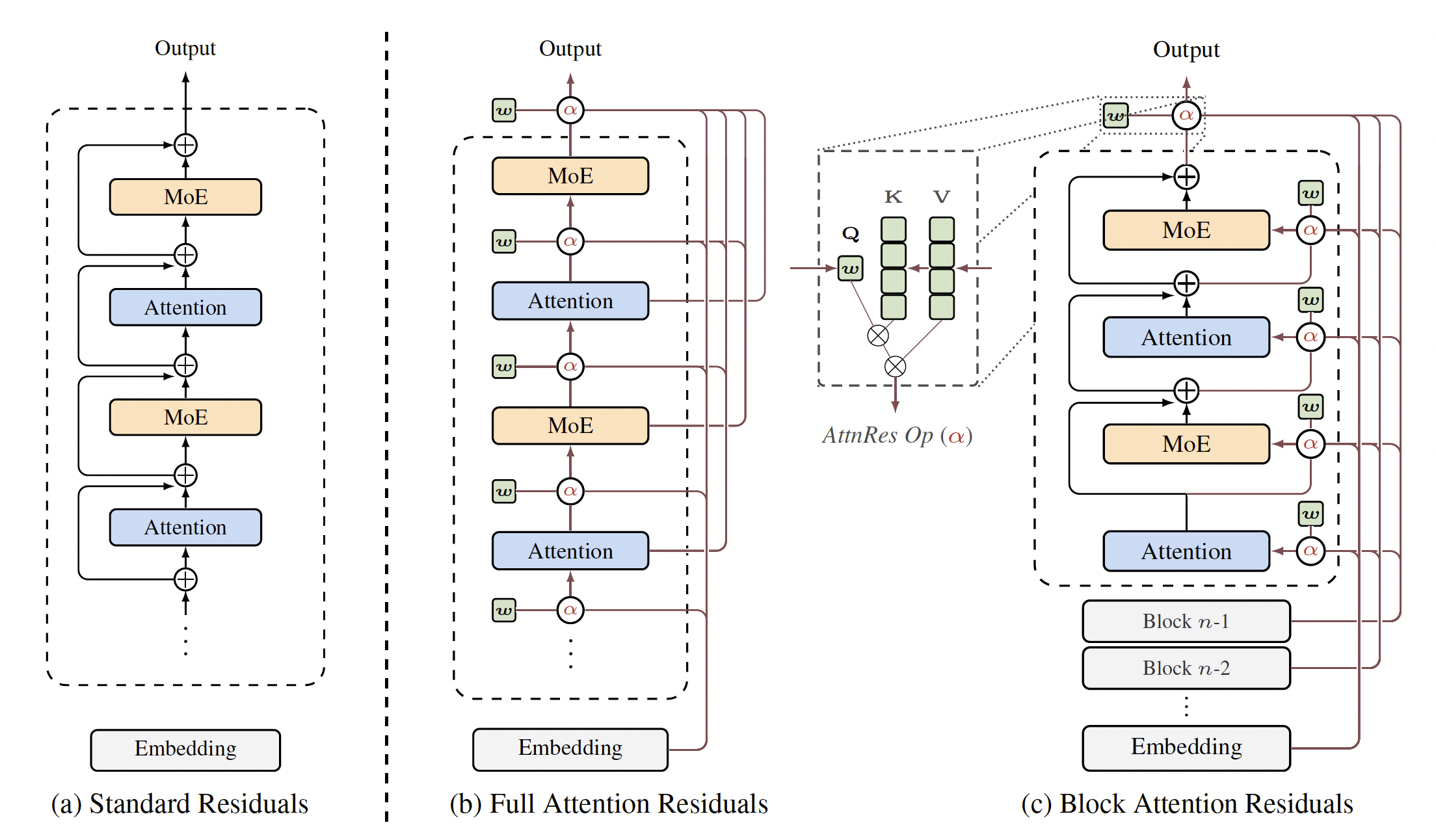
\[\begin{pmatrix}\phi(\boldsymbol{w}_1, \boldsymbol{y}_0) & & & \\\phi(\boldsymbol{w}_2, \boldsymbol{y}_0) & \phi(\boldsymbol{w}_2, \boldsymbol{y}_1) & & \\\phi(\boldsymbol{w}_3, \boldsymbol{y}_0) & \phi(\boldsymbol{w}_3, \boldsymbol{y}_{1:2}) & \phi(\boldsymbol{w}_3, \boldsymbol{y}_{1:2}) & \\\phi(\boldsymbol{w}_4, \boldsymbol{y}_0) & \phi(\boldsymbol{w}_4, \boldsymbol{y}_{1:3}) & \phi(\boldsymbol{w}_4, \boldsymbol{y}_{1:3}) & \phi(\boldsymbol{w}_4, \boldsymbol{y}_{1:3})\end{pmatrix}\]

The previous three architecture can be depicted as the following figure.

Main Results

Infra design

Block AttnRes needs to propagate the output across pipeline stages, causing heavy communication in a naive setting. Here we use a simple example to illustrate the idea.

The author used interleaved pipeline parallelism (PP) as a training setup (which mitigates the computational bubble problem of naive PP). Consider training a model with 8 layers on 2 GPUs, with 2 virtual stages per GPU:

• GPU 0 / Virtual Stage 0: Layers 1 & 2
• GPU 1 / Virtual Stage 0: Layers 3 & 4
• GPU 0 / Virtual Stage 1: Layers 5 & 6
• GPU 1 / Virtual Stage 1: Layers 7 & 8

First Pass (Virtual Stage 0): GPU 0 processes Layers 1 & 2, and creates the first completed block representation \(b_0\) which is cached in GPU 0. GPU 0 must transmit \(b_0\) to GPU 1 so it can process Layers 3 & 4 (\(b_1\)). Then \(b_0\) is cached in GPU 1’s local memory.

Second Pass (Virtual Stage 1): The pipeline loops back to GPU 0 to process Layers 5 & 6. GPU 0 receives a new block representation (\(b_1\)) and caches it. Now, GPU 0 needs to pass the data to GPU 1 for the final layers (7 & 8). Because of the caching optimization, GPU 0 only transmits the incremental new block (\(b_1\)) to GPU 1. It does not need to re-transmit \(b_0\), because GPU 1 already saved it during Virtual Stage 0.

Scaling law

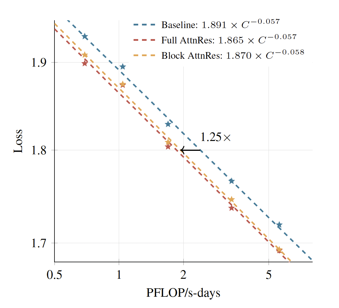
The authors trained a series of MoE models across five different sizes (active parameters 194M, 241M, 296M, 436M, and 528M, with total size from 3B to 48B). These models are based on the “Kimi Linear” architecture which mixes linear attention (Delta) and multi-head latent attention at ratio 3:1. All of these models were trained using an 8192-token context window.

“All three variants exhibit a similar slope, but AttnRes consistently achieves lower loss across the entire compute range.”

Training dynamics

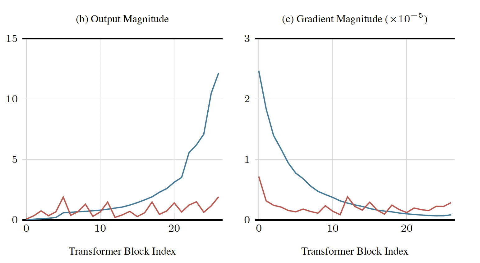
This plot shows the output and gradient magnitude across the layers of the transformer during training (blue: baseline, red: block AttnRes).

In the Baseline model, the size of hidden states grows continuously as the network gets deeper, which forces the deeper layers to produce increasingly large outputs. This leads to back-propagation having massive, disproportionate gradients in the earlier layers.

On the other hand, Block AttnRes keeps the output and gradient sizes bounded and periodic.

Conclusion

This paper (re)introduces the attention mechanism over the classic residual paradigm in a neural network. The idea is simple yet makes promising enhancements to transformer models. The major contribution beyond the idea is the implementation, which involves heavy engineering optimization. An expensive paper for sure.

Now transformers not only have attention along the sequence, but also attention across the layers. It feels complete.

References

• Kimi’s Attention Residual paper (2026)
• mHC: Manifold-Constrained Hyper-Connections - DeepSeek’s earlier work on residual connections
• Original mHC paper